Effective organization and description of data is a first step in most analyses. This section introduces the data matrix for organizing data as well as some terminology about different forms of data that will be used throughout this book.

Observations, variables, and data matrices

Figure 1.3 displays rows 1, 2, 3, and 50 of a data set for 50 randomly sampled loans offered through Lending Club, which is a peer-to-peer lending company. These observations will be referred to as the loan50 data set.

Each row in the table represents a single loan. The formal name for a row is a case or observational unit. The columns represent characteristics, called variables, for each of the loans. For example, the first row represents a loan of $22,000 with an interest rate of 10.90%, where the borrower is based in New Jersey (NJ) and has an income of $59,000.

Guided Practice 1.2

What is the grade of the first loan in Figure 1.3? And what is the home ownership status of the borrower for that first loan? For these Guided Practice questions, you can check your answer in the footnote.¹

In practice, it is especially important to ask clarifying questions to ensure important aspects of the data are understood. For instance, it is always important to be sure we know what each variable means and the units of measurement. Descriptions of the loan50 variables are given in Figure 1.4.

	`loan_amount`	`interest_rate`	`term`	`grade`	`state`	`total_income`	`homeownership`
1	22000	10.90	60.00	B	NJ	59000.00	rent
2	6000	9.92	36.00	B	CA	60000.00	rent
3	25000	26.30	36.00	E	SC	75000.00	mortgage
$\vdots$	$\vdots$	$\vdots$	$\vdots$	$\vdots$	$\vdots$	$\vdots$	$\vdots$
50	15000	6.08	36.00	A	TX	77500.00	mortgage

Figure 1.3. Four rows from the loan50 data matrix.

variable	description
`loan_amount`	Amount of the loan received, in US dollars.
`interest_rate`	Interest rate on the loan, in an annual percentage.
`term`	The length of the loan, which is always set as a whole number of months.
`grade`	Loan grade, which takes values A through G and represents the quality of the loan and its likelihood of being repaid.
`state`	US state where the borrower resides.
`total_income`	Borrower’s total income, including any second income, in US dollars.
`homeownership`	Indicates whether the person owns, owns but has a mortgage, or rents.

Figure 1.4. Variables and their descriptions for the loan50 data set.

The data in Figure 1.3 represent a data matrix, which is a convenient and common way to organize data, especially if collecting data in a spreadsheet. Each row of a data matrix corresponds to a unique case (observational unit), and each column corresponds to a variable.

When recording data, use a data matrix unless you have a very good reason to use a different structure. This structure allows new cases to be added as rows or new variables as new columns.

Guided Practice 1.3

The grades for assignments, quizzes, and exams in a course are often recorded in a gradebook that takes the form of a data matrix. How might you organize grade data using a data matrix?²

Guided Practice 1.4

We consider data for 3,142 counties in the United States, which includes each county’s name, the state where it resides, its population in 2017, how its population changed from 2010 to 2017, poverty rate, and six additional characteristics. How might these data be organized in a data matrix?³

The data described in Guided Practice 1.4 represents the county data set, which is shown as a data matrix in Figure 1.5. The variables are summarized in Figure 1.6.

	`name`	`state`	`pop`	`pop_change`	`poverty`	`homeownership`	`multi_unit`	`unemp_rate`	`metro`	`median_edu`	`median_hh_income`
1	Autauga	Alabama	55504	1.48	13.7	77.5	7.2	3.86	yes	some_college	55317
2	Baldwin	Alabama	212628	9.19	11.8	76.7	22.6	3.99	yes	some_college	52562
3	Barbour	Alabama	25270	-6.22	27.2	68.0	11.1	5.90	no	hs_diploma	33368
4	Bibb	Alabama	22668	0.73	15.2	82.9	6.6	4.39	yes	hs_diploma	43404
5	Blount	Alabama	58013	0.68	15.6	82.0	3.7	4.02	yes	hs_diploma	47412
6	Bullock	Alabama	10309	-2.28	28.5	76.9	9.9	4.93	no	hs_diploma	29655
7	Butler	Alabama	19825	-2.69	24.4	69.0	13.7	5.49	no	hs_diploma	36326
8	Calhoun	Alabama	114728	-1.51	18.6	70.7	14.3	4.93	yes	some_college	43686
9	Chambers	Alabama	33713	-1.20	18.8	71.4	8.7	4.08	no	hs_diploma	37342
10	Cherokee	Alabama	25857	-0.60	16.1	77.5	4.3	4.05	no	hs_diploma	40041
$\vdots$	$\vdots$	$\vdots$	$\vdots$	$\vdots$	$\vdots$	$\vdots$	$\vdots$	$\vdots$	$\vdots$	$\vdots$	$\vdots$
3142	Weston	Wyoming	6927	-2.93	14.4	77.9	6.5	3.98	no	some_college	59605

Figure 1.5. Eleven rows from the county data set.

variable	description
`name`	County name.
`state`	State where the county resides, or the District of Columbia.
`pop`	Population in 2017.
`pop_change`	Percent change in the population from 2010 to 2017. For example, the value `1.48` in the first row means the population for this county increased by 1.48% from 2010 to 2017.
`poverty`	Percent of the population in poverty.
`homeownership`	Percent of the population that lives in their own home or lives with the owner, e.g. children living with parents who own the home.
`multi_unit`	Percent of living units that are in multi-unit structures, e.g. apartments.
`unemp_rate`	Unemployment rate as a percent.
`metro`	Whether the county contains a metropolitan area.
`median_edu`	Median education level, which can take a value among `below_hs`, `hs_diploma`, `some_college`, and `bachelors`.
`median_hh_income`	Median household income for the county, where a household’s income equals the total income of its occupants who are 15 years or older.

Figure 1.6. Variables and their descriptions for the county data set.

Types of variables

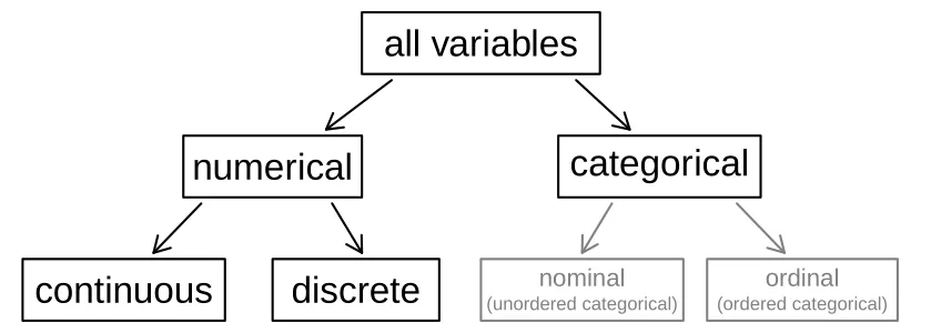
Examine the unemp_rate, pop, state, and median_edu variables in the county data set. Each of these variables is inherently different from the other three, yet some share certain characteristics.

First consider unemp_rate, which is said to be a numerical variable since it can take a wide range of numerical values, and it is sensible to add, subtract, or take averages with those values. On the other hand, we would not classify a variable reporting telephone area codes as numerical since the average, sum, and difference of area codes doesn’t have any clear meaning.

The pop variable is also numerical, although it seems to be a little different than unemp_rate. This variable of the population count can only take whole non-negative numbers (0, 1, 2, ...). For this reason, the population variable is said to be discrete since it can only take numerical values with jumps. On the other hand, the unemployment rate variable is said to be continuous.

The variable state can take up to 51 values after accounting for Washington, DC: AL, AK, ..., and WY. Because the responses themselves are categories, state is called a categorical variable, and the possible values are called the variable’s levels.

Finally, consider the median_edu variable, which describes the median education level of county residents and takes values below_hs, hs_diploma, some_college, or bachelors in each county. This variable seems to be a hybrid: it is a categorical variable but the levels have a natural ordering. A variable with these properties is called an ordinal variable, while a regular categorical variable without this type of special ordering is called a nominal variable. To simplify analyses, any ordinal variable in this book will be treated as a nominal (unordered) categorical variable.

Breakdown of variables into their respective types, showing "all variables" breaking down into "numeric" and "categorical". Then "numeric" is divided into "continuous" and "discrete", and "categorical" is broken down into "nominal (unordered categorical)" and "ordinal (ordered categorical)'' variables. — **Figure 1.7.** Breakdown of variables into their respective types.

Example 1.5

Data were collected about students in a statistics course. Three variables were recorded for each student: number of siblings, student height, and whether the student had previously taken a statistics course. Classify each of the variables as continuous numerical, discrete numerical, or categorical.

The number of siblings and student height represent numerical variables. Because the number of siblings is a count, it is discrete. Height varies continuously, so it is a continuous numerical variable. The last variable classifies students into two categories – those who have and those who have not taken a statistics course – which makes this variable categorical.

Guided Practice 1.6

An experiment is evaluating the effectiveness of a new drug in treating migraines. A group variable is used to indicate the experiment group for each patient: treatment or control. The num_migraines variable represents the number of migraines the patient experienced during a 3-month period. Classify each variable as either numerical or categorical.⁴

Relationships between variables

Many analyses are motivated by a researcher looking for a relationship between two or more variables. A social scientist may like to answer some of the following questions:

If homeownership is lower than the national average in one county, will the percent of multi-unit structures in that county tend to be above or below the national average?
Does a higher than average increase in county population tend to correspond to counties with higher or lower median household incomes?
How useful a predictor is median education level for the median household income for US counties?

To answer these questions, data must be collected, such as the county data set shown in Figure 1.5. Examining summary statistics could provide insights for each of the three questions about counties. Additionally, graphs can be used to visually explore data.

Scatterplots are one type of graph used to study the relationship between two numerical variables. Figure 1.8 compares the variables homeownership and multi_unit, which is the percent of units in multi-unit structures (e.g. apartments, condos). Each point on the plot represents a single county. For instance, the highlighted dot corresponds to County 413 in the county data set: Chattahoochee County, Georgia, which has 39.4% of units in multi-unit structures and a homeownership rate of 31.3%. The scatterplot suggests a relationship between the two variables: counties with a higher rate of multi-units tend to have lower homeownership rates. We might brainstorm as to why this relationship exists and investigate each idea to determine which are the most reasonable explanations.

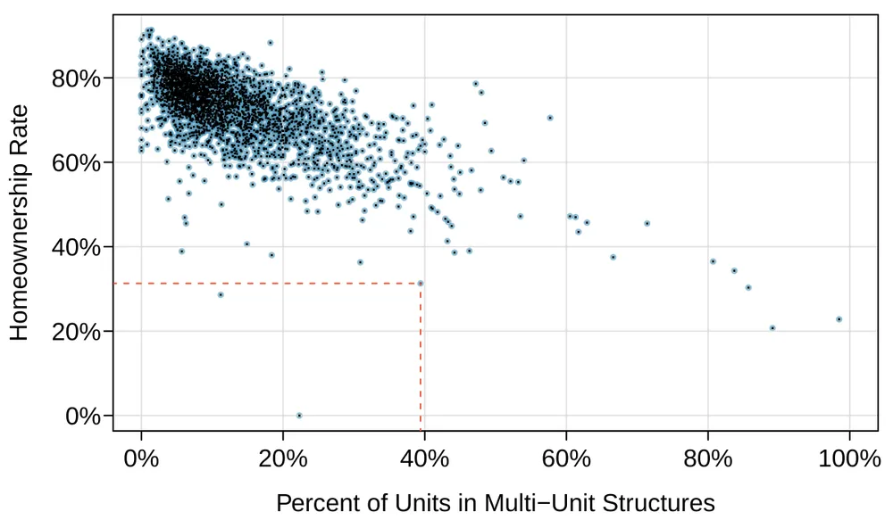
Scatterplot of thousands of counties with the percent of multiunit structures in each county shown on the horizontal axis and homeownership rate shown on the vertical axis. The data range from 0% to almost 100% for both variables. In general, the points are much more concentrated in the upper left corner of the graph and then trend downward for observations further to the right while also becoming more sparse. One point is annotated at the location (39.4%, 31.3.%). — **Figure 1.8.** A scatterplot of homeownership versus the percent of units that are in multi-unit structures for US counties. The highlighted dot represents Chattahoochee County, Georgia, which has a multi-unit rate of 39.4% and a homeownership rate of 31.3%.

The multi-unit and homeownership rates are said to be associated because the plot shows a discernible pattern. When two variables show some connection with one another, they are called associated variables. Associated variables can also be called dependent variables and vice-versa.

Guided Practice 1.7

Examine the variables in the loan50 data set, which are described in Figure 1.4. Create two questions about possible relationships between variables in loan50 that are of interest to you.⁵

Example 1.8

This example examines the relationship between a county’s population change from 2010 to 2017 and median household income, which is visualized as a scatterplot in Figure 1.9. Are these variables associated?

The larger the median household income for a county, the higher the population growth observed for the county. While this trend isn’t true for every county, the trend in the plot is evident. Since there is some relationship between the variables, they are associated.

Scatterplot of thousands of counties with the median household income along the horizontal axis (data ranging from 0 to 120,000) and population change over 7 years (data ranging from about -15% to 25%). There is a cloud of points centered around (45,000, -1%), and the points show a slight trend upwards while also becoming more sparse and volatile for observations corresponding to higher median incomes. One point is annotated at the location (22,736, -3.63%). 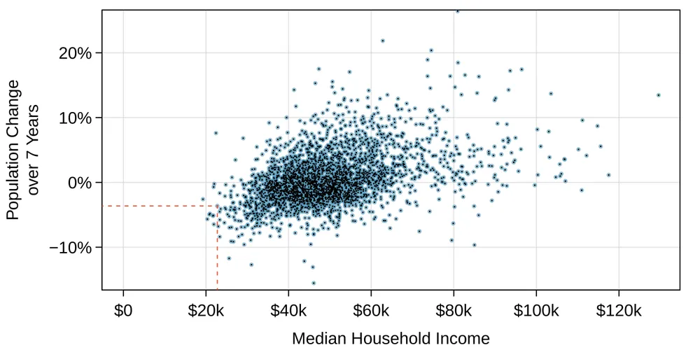— **Figure 1.9.** A scatterplot showing `pop_change` against `median_hh_income`. Owsley County of Kentucky, is highlighted, which lost 3.63% of its population from 2010 to 2017 and had median household income of $22,736.

Because there is a downward trend in Figure 1.8 – counties with more units in multi-unit structures are associated with lower homeownership – these variables are said to be negatively associated. A positive association is shown in the relationship between the median_hh_income and pop_change in Figure 1.9, where counties with higher median household income tend to have higher rates of population growth.

If two variables are not associated, then they are said to be independent. That is, two variables are independent if there is no evident relationship between the two.

Associated or independent, not both

A pair of variables are either related in some way (associated) or not (independent). No pair of variables is both associated and independent.

Explanatory and response variables

When we ask questions about the relationship between two variables, we sometimes also want to determine if the change in one variable causes a change in the other. Consider the following rephrasing of an earlier question about the county data set:

If there is an increase in the median household income in a county, does this drive an increase in its population?

In this question, we are asking whether one variable affects another. If this is our underlying belief, then median household income is the explanatory variable and the population change is the response variable in the hypothesized relationship.⁶

Explanatory and response variables

When we suspect one variable might causally affect another, we label the first variable the explanatory variable and the second the response variable.

Simple graphic shown the words "explanatory variable" pointing to "response variable", where the words "might affect" appear above the arrow.

For many pairs of variables, there is no hypothesized relationship, and these labels would not be applied to either variable in such cases.

Bear in mind that the act of labeling the variables in this way does nothing to guarantee that a causal relationship exists. A formal evaluation to check whether one variable causes a change in another requires an experiment.

Introducing observational studies and experiments

are two primary types of data collection: observational studies and experiments.

Researchers perform an observational study when they collect data in a way that does not directly interfere with how the data arise. For instance, researchers may collect information via surveys, review medical or company records, or follow a cohort of many similar individuals to form hypotheses about why certain diseases might develop. In each of these situations, researchers merely observe the data that arise. In general, observational studies can provide evidence of a naturally occurring association between variables, but they cannot by themselves show a causal connection.

When researchers want to investigate the possibility of a causal connection, they conduct an experiment. Usually there will be both an explanatory and a response variable. For instance, we may suspect administering a drug will reduce mortality in heart attack patients over the following year. To check if there really is a causal connection between the explanatory variable and the response, researchers will collect a sample of individuals and split them into groups. The individuals in each group are assigned a treatment. When individuals are randomly assigned to a group, the experiment is called a randomized experiment. For example, each heart attack patient in the drug trial could be randomly assigned, perhaps by flipping a coin, into one of two groups: the first group receives a placebo (fake treatment) and the second group receives the drug. See the case study in Section 1.1 for another example of an experiment, though that study did not employ a placebo.

Association $\neq$ Causation

In general, association does not imply causation, and causation can only be inferred from a randomized experiment.

Exercises

Exercise 1.3

Air pollution and birth outcomes, study components. Researchers collected data to examine the relationship between air pollutants and preterm births in Southern California. During the study air pollution levels were measured by air quality monitoring stations. Specifically, levels of carbon monoxide were recorded in parts per million, nitrogen dioxide and ozone in parts per hundred million, and coarse particulate matter (PM $_{10}$ ) in $\mu g/m^3$ . Length of gestation data were collected on 143,196 births between the years 1989 and 1993, and air pollution exposure during gestation was calculated for each birth. The analysis suggested that increased ambient PM $_{10}$ and, to a lesser degree, CO concentrations may be associated with the occurrence of preterm births.⁷

Identify the main research question of the study.
Who are the subjects in this study, and how many are included?
What are the variables in the study? Identify each variable as numerical or categorical. If numerical, state whether the variable is discrete or continuous. If categorical, state whether the variable is ordinal.

Exercise 1.4

Buteyko method, study components. The Buteyko method is a shallow breathing technique developed by Konstantin Buteyko, a Russian doctor, in 1952. Anecdotal evidence suggests that the Buteyko method can reduce asthma symptoms and improve quality of life. In a scientific study to determine the effectiveness of this method, researchers recruited 600 asthma patients aged 18-69 who relied on medication for asthma treatment. These patients were randomly split into two research groups: one practiced the Buteyko method and the other did not. Patients were scored on quality of life, activity, asthma symptoms, and medication reduction on a scale from 0 to 10. On average, the participants in the Buteyko group experienced a significant reduction in asthma symptoms and an improvement in quality of life.⁸

Identify the main research question of the study.
Who are the subjects in this study, and how many are included?
What are the variables in the study? Identify each variable as numerical or categorical. If numerical, state whether the variable is discrete or continuous. If categorical, state whether the variable is ordinal.

Exercise 1.5

Cheaters, study components. Researchers studying the relationship between honesty, age and self-control conducted an experiment on 160 children between the ages of 5 and 15. Participants reported their age, sex, and whether they were an only child or not. The researchers asked each child to toss a fair coin in private and to record the outcome (white or black) on a paper sheet, and said they would only reward children who report white. The study’s findings can be summarized as follows: “Half the students were explicitly told not to cheat and the others were not given any explicit instructions. In the no instruction group probability of cheating was found to be uniform across groups based on child’s characteristics. In the group that was explicitly told to not cheat, girls were less likely to cheat, and while rate of cheating didn’t vary by age for boys, it decreased with age for girls.”⁹

Identify the main research question of the study.
Who are the subjects in this study, and how many are included?
How many variables were recorded for each subject in the study in order to conclude these findings? State the variables and their types.

Exercise 1.6

Stealers, study components. In a study of the relationship between socio-economic class and unethical behavior, 129 University of California undergraduates at Berkeley were asked to identify themselves as having low or high social-class by comparing themselves to others with the most (least) money, most (least) education, and most (least) respected jobs. They were also presented with a jar of individually wrapped candies and informed that the candies were for children in a nearby laboratory, but that they could take some if they wanted. After completing some unrelated tasks, participants reported the number of candies they had taken.¹⁰

Identify the main research question of the study.
Who are the subjects in this study, and how many are included?
The study found that students who were identified as upper-class took more candy than others. How many variables were recorded for each subject in the study in order to conclude these findings? State the variables and their types.

Exercise 1.7

Migraine and acupuncture, Part II. Exercise 1.1 introduced a study exploring whether acupuncture had any effect on migraines. Researchers conducted a randomized controlled study where patients were randomly assigned to one of two groups: treatment or control. The patients in the treatment group received acupuncture that was specifically designed to treat migraines. The patients in the control group received placebo acupuncture (needle insertion at non-acupoint locations). 24 hours after patients received acupuncture, they were asked if they were pain free. What are the explanatory and response variables in this study?

Exercise 1.8

Sinusitis and antibiotics, Part II. Exercise 1.2 introduced a study exploring the effect of antibiotic treatment for acute sinusitis. Study participants either received either a 10-day course of an antibiotic (treatment) or a placebo similar in appearance and taste (control). At the end of the 10-day period, patients were asked if they experienced improvement in symptoms. What are the explanatory and response variables in this study?

Exercise 1.9

Fisher’s irises. Sir Ronald Aylmer Fisher was an English statistician, evolutionary biologist, and geneticist who worked on a data set that contained sepal length and width, and petal length and width from three species of iris flowers (setosa, versicolor and virginica). There were 50 flowers from each species in the data set. ¹¹

How many cases were included in the data?
How many numerical variables are included in the data? Indicate what they are, and if they are continuous or discrete.
How many categorical variables are included in the data, and what are they? List the corresponding levels (categories).

Photo by Ryan Claussen (http://flic.kr/p/6QTcuX) CC BY-SA 2.0 license

Exercise 1.10

Smoking habits of UK residents. A survey was conducted to study the smoking habits of UK residents. Below is a data matrix displaying a portion of the data collected in this survey. Note that “ $\pounds$ " stands for British Pounds Sterling, “cig" stands for cigarettes, and “N/A” refers to a missing component of the data. ¹²

	sex	age	marital	grossIncome	smoke	amtWeekends	amtWeekdays
1	Female	42	Single	Under $\pounds$ 2,600	Yes	12 cig/day	12 cig/day
2	Male	44	Single	$\pounds$ 10,400 to $\pounds$ 15,600	No	N/A	N/A
3	Male	53	Married	Above $\pounds$ 36,400	Yes	6 cig/day	6 cig/day
⋮	⋮	⋮	⋮	⋮	⋮	⋮	⋮
1691	Male	40	Single	$\pounds$ 2,600 to $\pounds$ 5,200	Yes	8 cig/day	8 cig/day

What does each row of the data matrix represent?
How many participants were included in the survey?
Indicate whether each variable in the study is numerical or categorical. If numerical, identify as continuous or discrete. If categorical, indicate if the variable is ordinal.

Exercise 1.11

US Airports. The visualization below shows the geographical distribution of airports in the contiguous United States and Washington, DC. This visualization was constructed based on a dataset where each observation is an airport.¹³

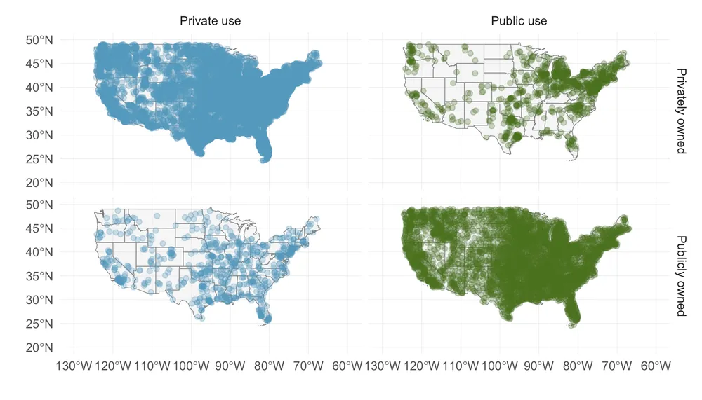
List the variables used in creating this visualization.
Indicate whether each variable in the study is numerical or categorical. If numerical, identify as continuous or discrete. If categorical, indicate if the variable is ordinal.

Exercise 1.12

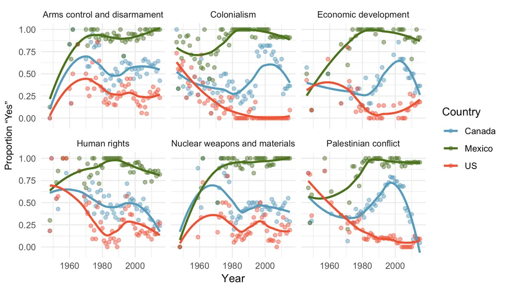
UN Votes. The visualization below shows voting patterns in the United States, Canada, and Mexico in the United Nations General Assembly on a variety of issues. Specifically, for a given year between 1946 and 2015, it displays the percentage of roll calls in which the country voted yes for each issue. This visualization was constructed based on a dataset where each observation is a country/year pair.¹⁴

List the variables used in creating this visualization.
Indicate whether each variable in the study is numerical or categorical. If numerical, identify as continuous or discrete. If categorical, indicate if the variable is ordinal.

Notes

The loan’s grade is B, and the borrower rents their residence. ↩
Each county may be viewed as a case, and there are eleven pieces of information recorded for each case. A table with 3,142 rows and 11 columns could hold these data, where each row represents a county and each column represents a particular piece of information. ↩
There are multiple strategies that can be followed. One common strategy is to have each student represented by a row, and then add a column for each assignment, quiz, or exam. Under this setup, it is easy to review a single line to understand a student’s grade history. There should also be columns to include student information, such as one column to list student names. ↩
The group variable can take just one of two group names, making it categorical. The num_migraines variable describes a count of the number of migraines, which is an outcome where basic arithmetic is sensible, which means this is numerical outcome; more specifically, since it represents a count, num_migraines is a discrete numerical variable. ↩
Two example questions: (1) What is the relationship between loan amount and total income? (2) If someone’s income is above the average, will their interest rate tend to be above or below the average? ↩
Sometimes the explanatory variable is called the independent variable and the response variable is called the dependent variable. However, this becomes confusing since a pair of variables might be independent or dependent, so we avoid this language. ↩
Ritz, B. et al. Effect of air pollution on preterm birth among children born in Southern California between 1989 and 1993. Epidemiology. 2000. ↩
McGowan, J. Health Education: Does the Buteyko Institute Method make a difference?. Thorax. 2003. ↩
Bucciol, Alessandro and Piovesan, Marco. Luck or cheating? A field experiment on honesty with children. Journal of Economic Psychology. 2011. ↩
Piff, P.K. et al. Higher social class predicts increased unethical behavior. Proceedings of the National Academy of Sciences. 2012. ↩
Fisher, R.A. The Use of Multiple Measurements in Taxonomic Problems. Annals of Eugenics. 1936. ↩
National STEM Centre, Large Datasets from stats4schools. ↩
Federal Aviation Administration, www.faa.gov/airports/airport_safety/airportdata_5010. ↩
David Robinson. unvotes: United Nations General Assembly Voting Data. R package version 0.2.0. 2017. ↩

Build status · Flash Infinity AI™ is a trademark of AI-Flash Inc.. WorldClass is not affiliated with, approved or accredited by any exam board, curriculum provider or university unless a page says so.

Data basics