WorldClass Statistics · Introduction to linear regression

Chapter 8 exercises

Exercise 8.37

True / False. Determine if the following statements are true or false. If false, explain why.

  1. A correlation coefficient of -0.90 indicates a stronger linear relationship than a correlation of 0.5.

  2. Correlation is a measure of the association between any two variables.

Exercise 8.38

Trees. The scatterplots below show the relationship between height, diameter, and volume of timber in 31 felled black cherry trees. The diameter of the tree is measured 4.5 feet above the ground.1
A scatterplot is shown with around 30 points. The horizontal axis is for "Height, in feet" and takes values between 60 and 90 feet. The vertical axis is for "Volume, in cubic feet" and takes values between 8 and 80 cubic feet. For the five points with heights smaller than 70 feet, volumes range from about 8 to 25 cubic feet. For the fifteen points with heights between 70 and 80 feet, volumes mostly range from about 15 to 50 cubic feet. For the ten points with heights larger than 80 feet, volumes mostly range from about 20 to 65 cubic feet, with one outlier with a height of about 88 feet and a volume of about 80 cubic feet. A scatterplot is shown with around 30 points. The horizontal axis is for "Diameter, in inches" and takes values between 8 and 22 inches. The vertical axis is for "Volume, in cubic feet" and takes values between 8 and 80 cubic feet. About 15 points with circumferences smaller than 12 inches, volumes range from about 8 to 25 cubic feet. For the approximately ten points with circumferences between 12 and 16 feet, volumes range from 22 to 35 cubic feet. For the 6 points with circumferences larger than 16 inches, volumes range from 40 to 60 cubic feet, with one outlier with a circumference of 22 inches and a volume of about 80 cubic feet.

  1. Describe the relationship between volume and height of these trees.

  2. Describe the relationship between volume and diameter of these trees.

  3. Suppose you have height and diameter measurements for another black cherry tree. Which of these variables would be preferable to use to predict the volume of timber in this tree using a simple linear regression model? Explain your reasoning.

Exercise 8.39

Husbands and wives, Part III. Exercise 8.33 presents a scatterplot displaying the relationship between husbands’ and wives’ ages in a random sample of 170 married couples in Britain, where both partners’ ages are below 65 years. Given below is summary output of the least squares fit for predicting wife’s age from husband’s age.
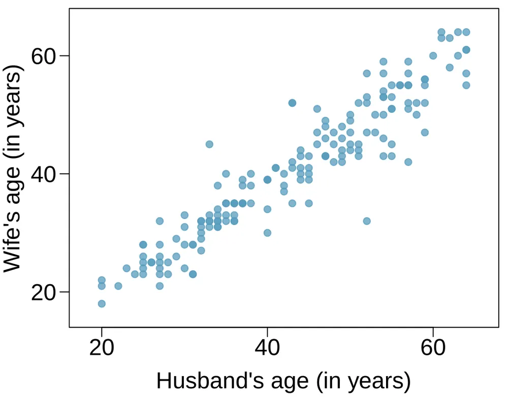
A scatterplot is shown with about 150 points. The horizontal axis is for "Hus, in inches" and takes values between 8 and 22 inches. The vertical axis is for "Volume, in cubic feet" and takes values between 8 and 80 cubic feet. About 15 points with circumferences smaller than 12 inches, volumes range from about 8 to 25 cubic feet. For the approximately ten points with circumferences between 12 and 16 feet, volumes range from 22 to 35 cubic feet. For the 6 points with circumferences larger than 16 inches, volumes range from 40 to 60 cubic feet, with one outlier with a circumference of 22 inches and a volume of about 80 cubic feet.

Estimate Std. Error t value Pr(>>∣|t∣|)
(Intercept) 1.5740 1.1501 1.37 0.1730
age_husband 0.9112 0.0259 35.25 0.0000
df=168df = 168
  1. We might wonder, is the age difference between husbands and wives consistent across ages? If this were the case, then the slope parameter would be β1=1\beta_1 = 1. Use the information above to evaluate if there is strong evidence that the difference in husband and wife ages differs for different ages.

  2. Write the equation of the regression line for predicting wife’s age from husband’s age.

  3. Interpret the slope and intercept in context.

  4. Given that R2=0.88R^2 = 0.88, what is the correlation of ages in this data set?

  5. You meet a married man from Britain who is 55 years old. What would you predict his wife’s age to be? How reliable is this prediction?

  6. You meet another married man from Britain who is 85 years old. Would it be wise to use the same linear model to predict his wife’s age? Explain.

Exercise 8.40

Cats, Part II. Exercise 8.26 presents regression output from a model for predicting the heart weight (in g) of cats from their body weight (in kg). The coefficients are estimated using a dataset of 144 domestic cat. The model output is also provided below.

Estimate Std. Error t value Pr(>>∣|t∣|)
(Intercept) -0.357 0.692 -0.515 0.607
body wt 4.034 0.250 16.119 0.000

s=1.452R2=64.66%Radj2=64.41%s = 1.452 \qquad R^2 = 64.66\% \qquad R^2_{adj} = 64.41\%

  1. We see that the point estimate for the slope is positive. What are the hypotheses for evaluating whether body weight is positively associated with heart weight in cats?

  2. State the conclusion of the hypothesis test from part (a) in context of the data.

  3. Calculate a 95% confidence interval for the slope of body weight, and interpret it in context of the data.

  4. Do your results from the hypothesis test and the confidence interval agree? Explain.

Exercise 8.41

Nutrition at Starbucks, Part II. Exercise 8.22 introduced a data set on nutrition information on Starbucks food menu items. Based on the scatterplot and the residual plot provided, describe the relationship between the protein content and calories of these menu items, and determine if a simple linear model is appropriate to predict amount of protein from the number of calories.
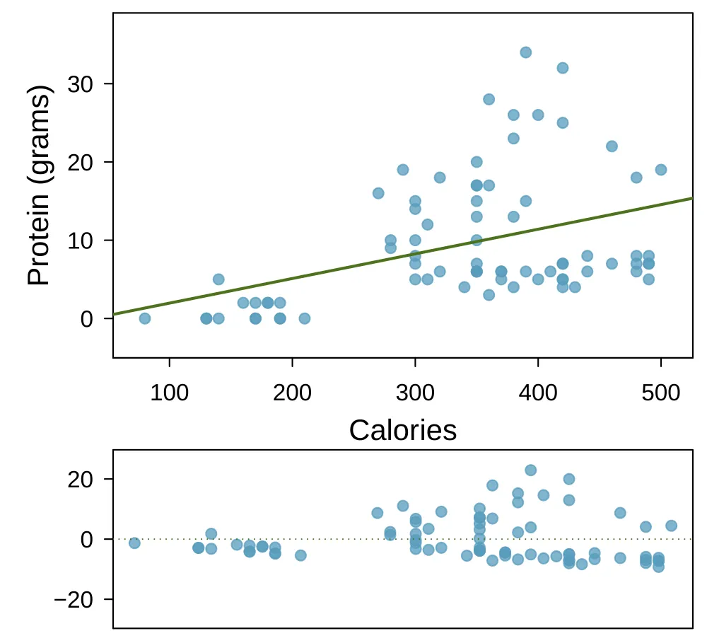
A scatterplot is shown with about 75 points and an overlaid regression line that trends upward along with a residual plot. The horizontal axis represents "Calories" and has values ranging from about 100 to 500. The vertical axis represents "Protein, in grams" and has values ranging from 0 to about 30. Scatterplot: About 15 points are shown with fewer than 200 calories, and these have between about 0 and 5 grams of protein. About 30 points are shown with 200 to 400 calories, and these mostly have between 5 and 30 grams of protein. About 20 points are shown with more than 400 calories, and these mostly have between 5 and 30 grams of carbs. Residual plot: About 15 points are shown with fewer than 200 calories, and these have residuals roughly between -5 and positive 2. About 30 points are shown with 200 to 400 calories, and these residuals largely range from about -10 to positive 20. About 20 points are shown with more than 400 calories, and the residuals for these points mostly range between -10 and positive 8.

Exercise 8.42

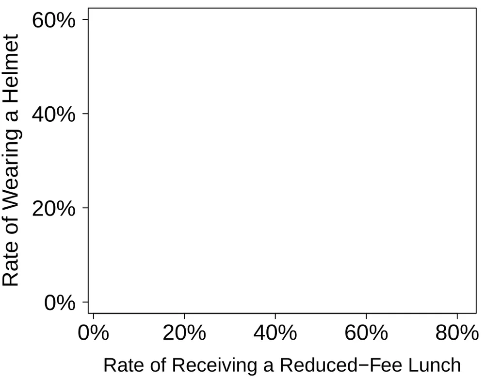
Helmets and lunches. The scatterplot shows the relationship between socioeconomic status measured as the percentage of children in a neighborhood receiving reduced-fee lunches at school (lunch) and the percentage of bike riders in the neighborhood wearing helmets (helmet). The average percentage of children receiving reduced-fee lunches is 30.8% with a standard deviation of 26.7% and the average percentage of bike riders wearing helmets is 38.8% with a standard deviation of 16.9%.

  1. If the R2R^2 for the least-squares regression line for these data is 72%72\%, what is the correlation between lunch and helmet?

  2. Calculate the slope and intercept for the least-squares regression line for these data.

  3. Interpret the intercept of the least-squares regression line in the context of the application.

  4. Interpret the slope of the least-squares regression line in the context of the application.

  5. What would the value of the residual be for a neighborhood where 40% of the children receive reduced-fee lunches and 40% of the bike riders wear helmets? Interpret the meaning of this residual in the context of the application.
 \:

A scatterplot is shown with 12 points. The horizontal axis is for "Rate of Receiving a Reduced-Fee Lunch" and takes values between 0% and 82%. The vertical axis is for "Rate of Wearing a Helmet" and takes values between about 3% and 58%. Eight points have a reduced-fee lunch rate smaller than 25%, and these points have helmet wearing rates between about 20% and 58%. Two points have a reduced-fee lunch rate of about 50%, and these points have helmet wearing rates about 21% and 22%. Two points have a reduced-fee lunch rate of 75% and 82%, and these points have helmet wearing rates of 5% and 3%, respectively.

Exercise 8.43

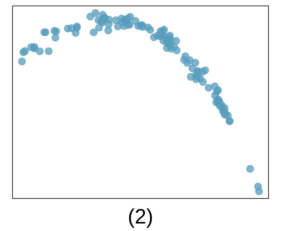
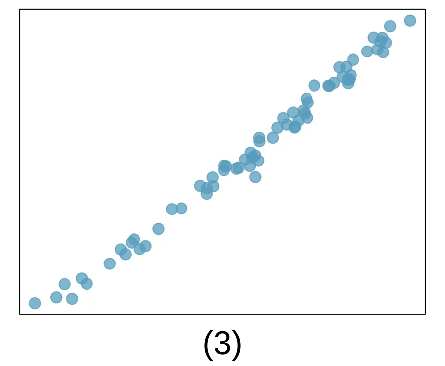
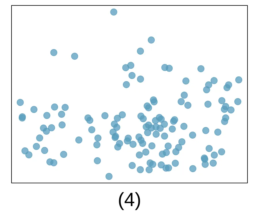
Match the correlation, Part III. Match each correlation to the corresponding scatterplot.
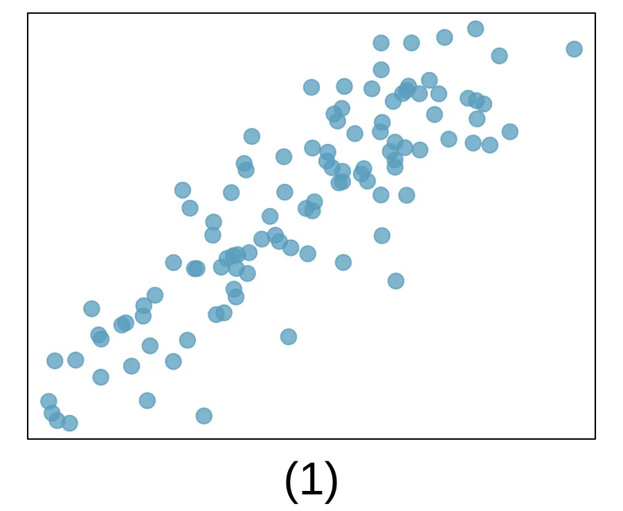
  1. r=−0.72r = -0.72

  2. r=0.07r = 0.07

  3. r=0.86r = 0.86

  4. r=0.99r = 0.99

A scatterplot is shown. The left third of the data has values that range in the bottom half of the range in the vertical direction. The middle third of the data has values that mostly range in the middle 50% of the vertical direction. The right third of the data has values that range in the upper half of the range in the vertical direction. A scatterplot is shown. The pattern resembles an arch, where the left third of the arch has been cut off. The peak of this "arch" of data is about a third of the way into the horizontal range. A scatterplot is shown, with what appears to be a stable upward trend in the data. If we were to imagine a line drawn against the data, the residuals would generally have a standard deviation equal to only about 5% of the vertical range of the data. That is, the data would be very "tightly packed" around the regression line. A scatterplot is shown. There is no clear pattern in the data when looking from left to right.

Exercise 8.44

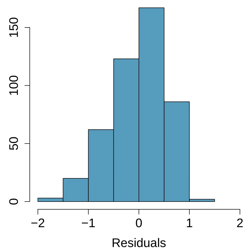
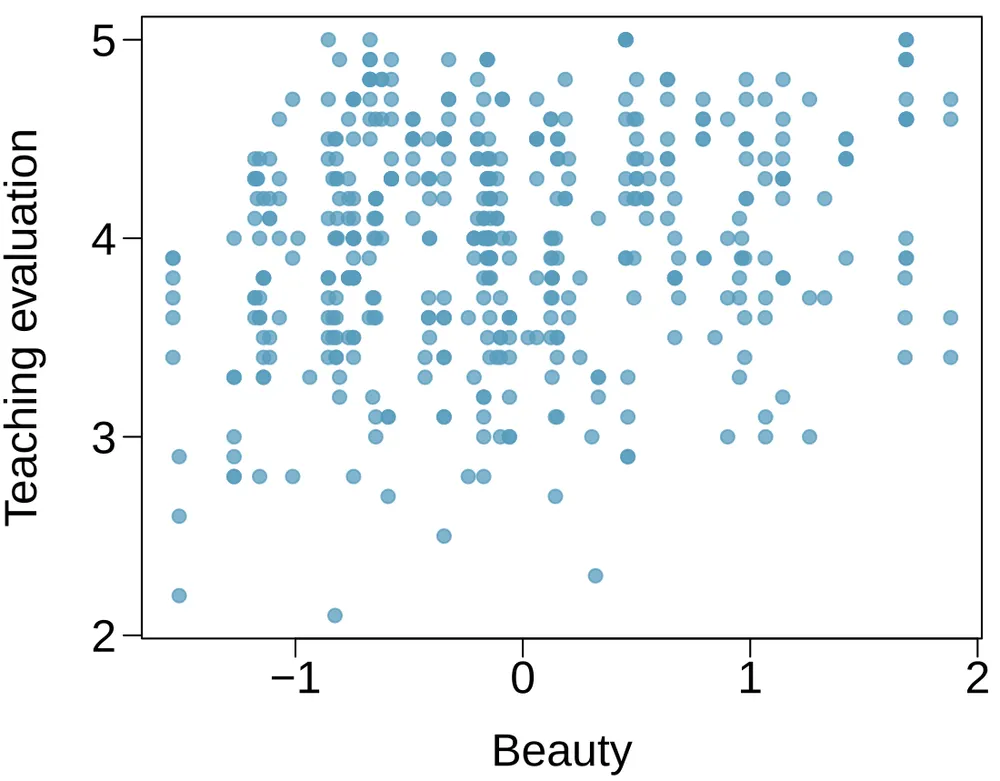
Rate my professor. Many college courses conclude by giving students the opportunity to evaluate the course and the instructor anonymously. However, the use of these student evaluations as an indicator of course quality and teaching effectiveness is often criticized because these measures may reflect the influence of non-teaching related characteristics, such as the physical appearance of the instructor. Researchers at University of Texas, Austin collected data on teaching evaluation score (higher score means better) and standardized beauty score (a score of 0 means average, negative score means below average, and a positive score means above average) for a sample of 463 professors.2 The scatterplot below shows the relationship between these variables, and regression output is provided for predicting teaching evaluation score from beauty score.

Estimate Std. Error t value Pr(>>∣|t∣|)
(Intercept) 4.010 0.0255 157.21 0.0000
beauty Cell 1 0.0322 4.13 0.0000
  1. Given that the average standardized beauty score is -0.0883 and average teaching evaluation score is 3.9983, calculate the slope. Alternatively, the slope may be computed using just the information provided in the model summary table.

  2. Do these data provide convincing evidence that the slope of the relationship between teaching evaluation and beauty is positive? Explain your reasoning.

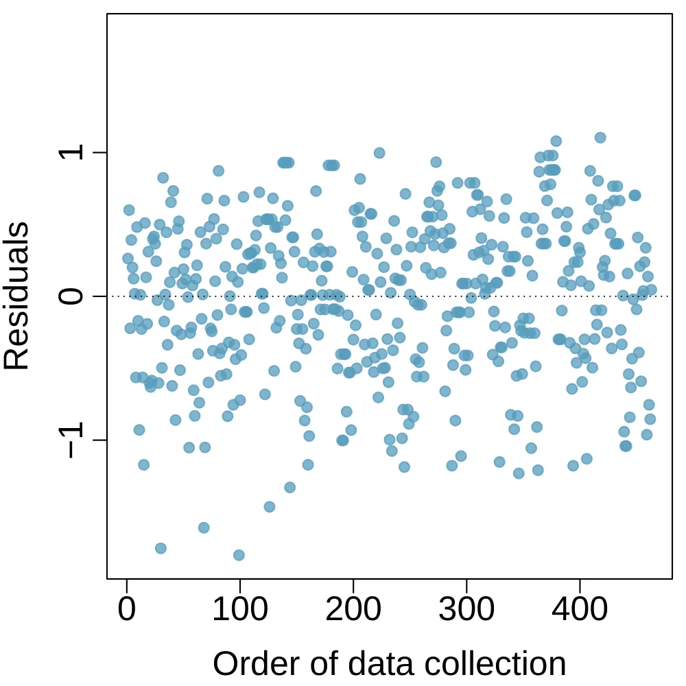
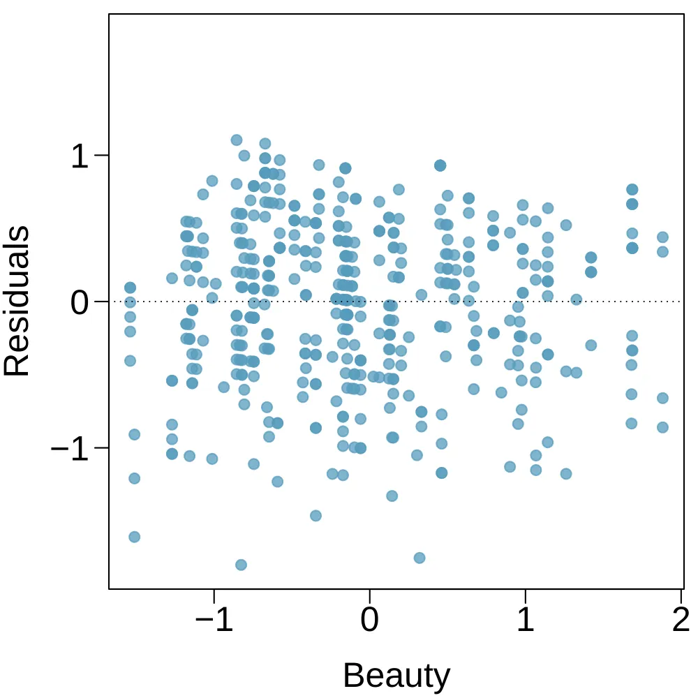
  3. List the conditions required for linear regression and check if each one is satisfied for this model based on the following diagnostic plots.
 \:

A scatterplot is shown for several hundred points. The horizontal axis is for a "Beauty" score and takes values between -1.8 and positive 2. The vertical axis is for "Teaching evaluation" and takes values between 2 and 5. For beauty scores smaller than 0, the Teaching Evaluation scores range mostly between 2.5 and 4.8, with no obvious trend in this region of the data. For beauty scores between 0 and 1, the Teaching Evaluation scores range mostly between 3 and 4.7. For beauty scores between 1 and 2, the Teaching Evaluation scores range mostly between 3.2 and 4.8.

A residual plot is shown for several hundred points. The horizontal axis is for a "Beauty" score and takes values between -1.8 and positive 2. The vertical axis is for "Residuals" and takes values between -1.5 and positive 1. For beauty scores smaller than 0, the residuals range mostly between -1.2 and positive 1. For beauty scores between 0 and 1, the residuals range mostly between -1.2 and positive 0.8. For beauty scores between 1 and 2, which has somewhat fewer points, the residuals range mostly between -1.0 and positive 0.5. A histogram is shown for residuals, where bins range between -2 and 1.5. The distribution is centered at zero and very slightly skewed to the left. A scatterplot is shown. The horizontal axis is for "Order of data collection" and takes values between 1 and about 450. The vertical axis is for "Residuals" and takes values between about -1.5 and positive 1. The residuals mostly lie between -1.2 and 0.9 across the range with no discernible pattern.

Notes

  1. Source: R Dataset, stat.ethz.ch/R-manual/R-patched/library/datasets/html/trees.html. ↩

  2. Hamermesh, Daniel S and Parker, Amy. Beauty in the classroom: Instructors’ pulchritude and putative pedagogical productivity. Economics of Education Review. 2005. ↩

Credit and licence

“Chapter 8 exercises” is from OpenIntro Statistics, Fourth Edition, by David M Diez, Mine Çetinkaya-Rundel and Christopher D Barr, shared under a CC BY-SA 3.0 license. WorldClass Statistics is a derivative of OpenIntro Statistics, shared under the same license; the original book may be found at openintro.org/book/os.

Source: https://www.openintro.org/book/os/

Licence: CC BY-SA 3.0 (creativecommons.org/licenses/by-sa/3.0/). You may share and adapt it under the same licence, with this credit. WorldClass adapted the formatting only: the text is the authors', with interactive parts and links to other sites left out.

Build status · Flash Infinity AI™ is a trademark of AI-Flash Inc.. WorldClass is not affiliated with, approved or accredited by any exam board, curriculum provider or university unless a page says so.