Linear regression is a very powerful statistical technique. Many people have some familiarity with regression just from reading the news, where straight lines are overlaid on scatterplots. Linear models can be used for prediction or to evaluate whether there is a linear relationship between two numerical variables.
It’s helpful to think deeply about the line fitting process. In this section, we define the form of a linear model, explore criteria for what makes a good fit, and introduce a new statistic called correlation.
Fitting a line to data
Figure 8.1 shows two variables whose relationship can be modeled perfectly with a straight line. The equation for the line is Consider what a perfect linear relationship means: we know the exact value of just by knowing the value of . This is unrealistic in almost any natural process. For example, if we took family income (), this value would provide some useful information about how much financial support a college may offer a prospective student (). However, the prediction would be far from perfect, since other factors play a role in financial support beyond a family’s finances.
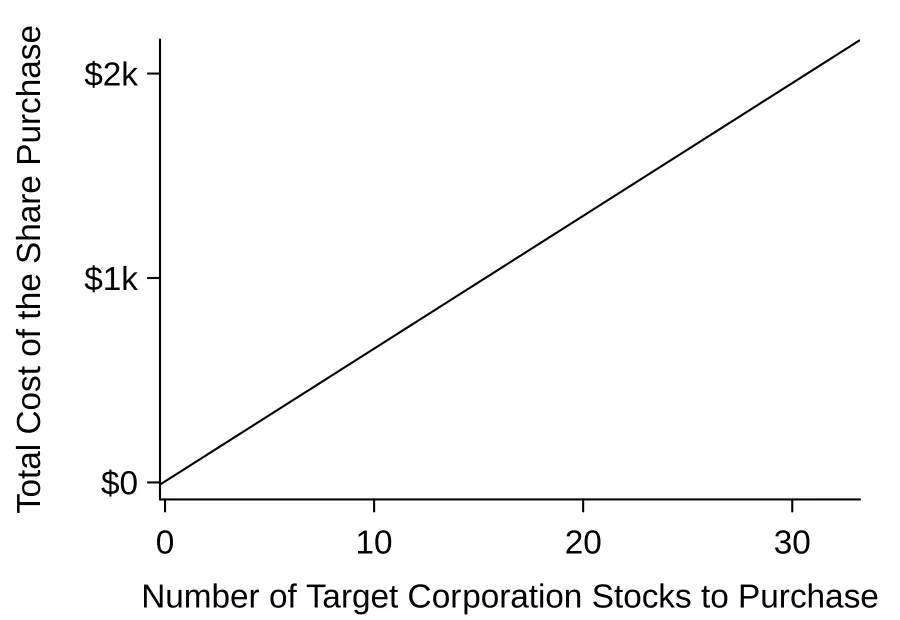
TGT, December 28th, 2018), and the total cost of the shares were reported. Because the cost is computed using a linear formula, the linear fit is perfect.Linear regression is the statistical method for fitting a line to data where the relationship between two variables, and , can be modeled by a straight line with some error: The values and represent the model’s parameters ( is the Greek letter beta), and the error is represented by (the Greek letter epsilon). The parameters are estimated using data, and we write their point estimates as and . When we use to predict , we usually call the explanatory or predictor variable, and we call the response; we also often drop the term when writing down the model since our main focus is often on the prediction of the average outcome.
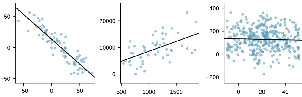
It is rare for all of the data to fall perfectly on a straight line. Instead, it’s more common for data to appear as a cloud of points, such as those examples shown in Figure 8.2. In each case, the data fall around a straight line, even if none of the observations fall exactly on the line. The first plot shows a relatively strong downward linear trend, where the remaining variability in the data around the line is minor relative to the strength of the relationship between and . The second plot shows an upward trend that, while evident, is not as strong as the first. The last plot shows a very weak downward trend in the data, so slight we can hardly notice it. In each of these examples, we will have some uncertainty regarding our estimates of the model parameters, and . For instance, we might wonder, should we move the line up or down a little, or should we tilt it more or less? As we move forward in this chapter, we will learn about criteria for line-fitting, and we will also learn about the uncertainty associated with estimates of model parameters.
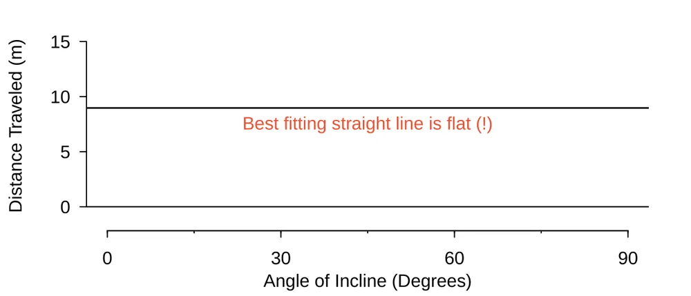
There are also cases where fitting a straight line to the data, even if there is a clear relationship between the variables, is not helpful. One such case is shown in Figure 8.3 where there is a very clear relationship between the variables even though the trend is not linear. We discuss nonlinear trends in this chapter and the next, but details of fitting nonlinear models are saved for a later course.
Using linear regression to predict possum head lengths
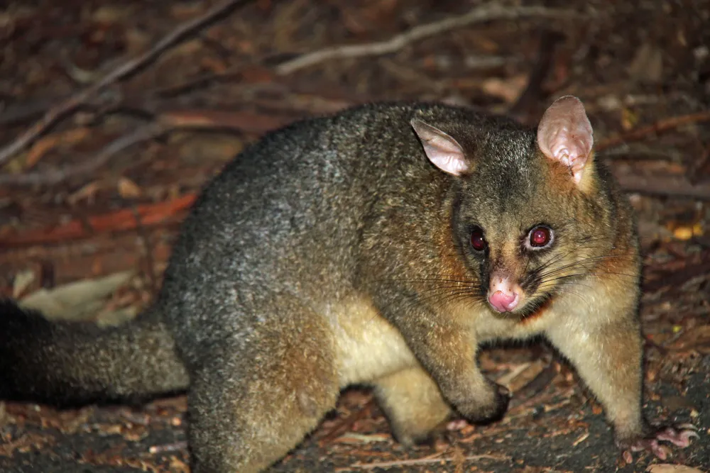
Brushtail possums are a marsupial that lives in Australia, and a photo of one is shown in Figure 8.4. Researchers captured 104 of these animals and took body measurements before releasing the animals back into the wild. We consider two of these measurements: the total length of each possum, from head to tail, and the length of each possum’s head.
—————————–
Photo by Greg Schechter (https://flic.kr/p/9BAFbR). CC BY 2.0 license.
Figure 8.5 shows a scatterplot for the head length and total length of the possums. Each point represents a single possum from the data. The head and total length variables are associated: possums with an above average total length also tend to have above average head lengths. While the relationship is not perfectly linear, it could be helpful to partially explain the connection between these variables with a straight line.
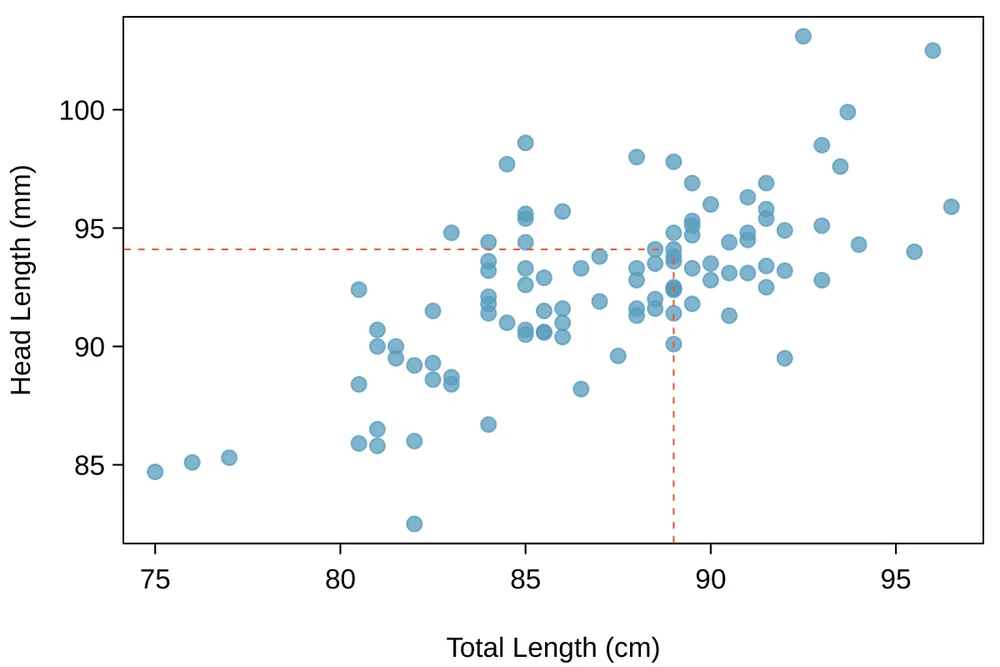
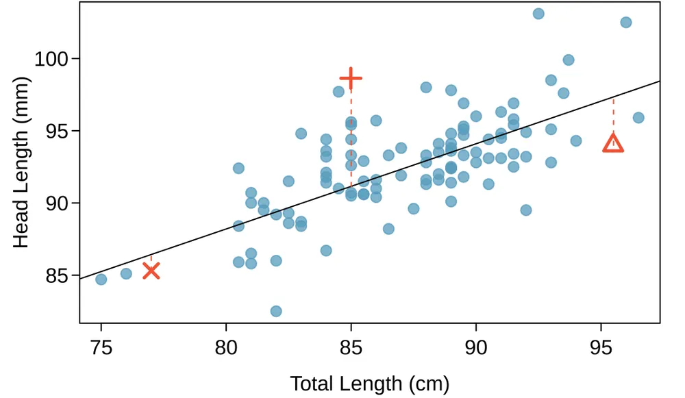
We want to describe the relationship between the head length and total length variables in the possum data set using a line. In this example, we will use the total length as the predictor variable, , to predict a possum’s head length, . We could fit the linear relationship by eye, as in Figure 8.6. The equation for this line is A “hat” on is used to signify that this is an estimate. We can use this line to discuss properties of possums. For instance, the equation predicts a possum with a total length of 80 cm will have a head length of The estimate may be viewed as an average: the equation predicts that possums with a total length of 80 cm will have an average head length of 88.2 mm. Absent further information about an 80 cm possum, the prediction for head length that uses the average is a reasonable estimate.
Example 8.1
What other variables might help us predict the head length of a possum besides its length?
Perhaps the relationship would be a little different for male possums than female possums, or perhaps it would differ for possums from one region of Australia versus another region. In Chapter 9, we’ll learn about how we can include more than one predictor. Before we get there, we first need to better understand how to best build a simple linear model with one predictor.
Residuals
Residuals are the leftover variation in the data after accounting for the model fit: Each observation will have a residual, and three of the residuals for the linear model we fit for the possum data is shown in Figure 8.6. If an observation is above the regression line, then its residual, the vertical distance from the observation to the line, is positive. Observations below the line have negative residuals. One goal in picking the right linear model is for these residuals to be as small as possible.
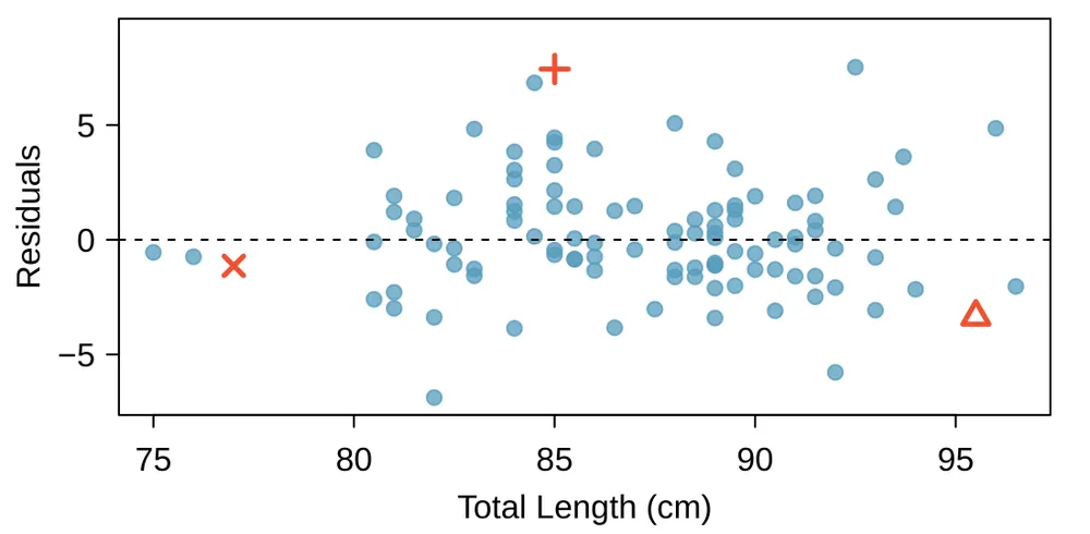
Let’s look closer at the three residuals featured in Figure 8.6. The observation marked by an “” has a small, negative residual of about -1; the observation marked by “” has a large residual of about +7; and the observation marked by “” has a moderate residual of about -4. The size of a residual is usually discussed in terms of its absolute value. For example, the residual for “” is larger than that of “” because is larger than .
Residual: difference between observed and expected
The residual of the observation is the difference of the observed response () and the response we would predict based on the model fit (): We typically identify by plugging into the model.
Example 8.2
The linear fit shown in Figure 8.6 is given as . Based on this line, formally compute the residual of the observation . This observation is denoted by “” in Figure 8.6. Check it against the earlier visual estimate, -1.
We first compute the predicted value of point “” based on the model: Next we compute the difference of the actual head length and the predicted head length: The model’s error is mm, which is very close to the visual estimate of -1mm. The negative residual indicates that the linear model overpredicted head length for this particular possum.
Guided Practice 8.3
If a model underestimates an observation, will the residual be positive or negative? What about if it overestimates the observation?1
Guided Practice 8.4
Compute the residuals for the “” observation and the “” observation in the figure using the linear relationship .2
Residuals are helpful in evaluating how well a linear model fits a data set. We often display them in a residual plot such as the one shown in Figure 8.7 for the regression line in Figure 8.6. The residuals are plotted at their original horizontal locations but with the vertical coordinate as the residual. For instance, the point had a residual of 7.45, so in the residual plot it is placed at . Creating a residual plot is sort of like tipping the scatterplot over so the regression line is horizontal.
Example 8.5
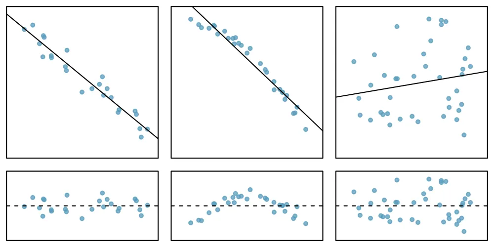
One purpose of residual plots is to identify characteristics or patterns still apparent in data after fitting a model. Figure 8.8 shows three scatterplots with linear models in the first row and residual plots in the second row. Can you identify any patterns remaining in the residuals?
In the first data set (first column), the residuals show no obvious patterns. The residuals appear to be scattered randomly around the dashed line that represents 0.
The second data set shows a pattern in the residuals. There is some curvature in the scatterplot, which is more obvious in the residual plot. We should not use a straight line to model these data. Instead, a more advanced technique should be used.
The last plot shows very little upwards trend, and the residuals also show no obvious patterns. It is reasonable to try to fit a linear model to the data. However, it is unclear whether there is statistically significant evidence that the slope parameter is different from zero. The point estimate of the slope parameter, labeled , is not zero, but we might wonder if this could just be due to chance. We will address this sort of scenario in Section 8.4.
Describing linear relationships with correlation
’ve seen plots with strong linear relationships and others with very weak linear relationships. It would be useful if we could quantify the strength of these linear relationships with a statistic.
Correlation: strength of a linear relationship
Correlation, which always takes values between -1 and 1, describes the strength of the linear relationship between two variables. We denote the correlation by .
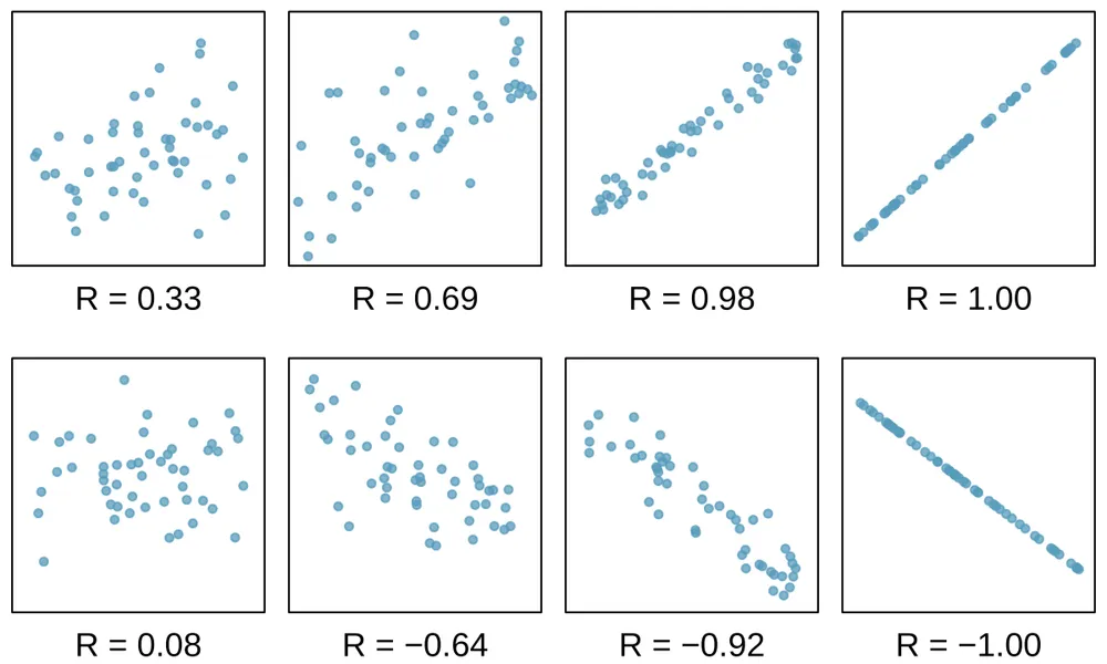
We can compute the correlation using a formula, just as we did with the sample mean and standard deviation. This formula is rather complex,3 and like with other statistics, we generally perform the calculations on a computer or calculator. Figure 8.9 shows eight plots and their corresponding correlations. Only when the relationship is perfectly linear is the correlation either -1 or 1. If the relationship is strong and positive, the correlation will be near +1. If it is strong and negative, it will be near -1. If there is no apparent linear relationship between the variables, then the correlation will be near zero.
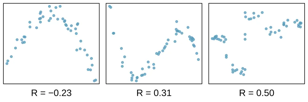
The correlation is intended to quantify the strength of a linear trend. Nonlinear trends, even when strong, sometimes produce correlations that do not reflect the strength of the relationship; see three such examples in Figure 8.10.
Guided Practice 8.6
No straight line is a good fit for the data sets represented in Figure 8.10. Try drawing nonlinear curves on each plot. Once you create a curve for each, describe what is important in your fit.4
Exercises
Exercise 8.1
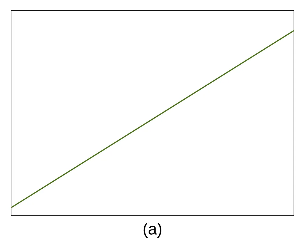
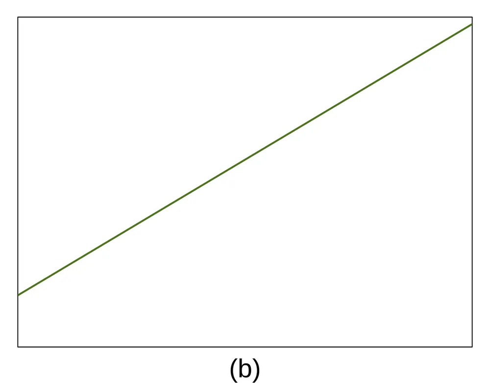
Visualize the residuals. The scatterplots shown below each have a superimposed regression line. If we were to construct a residual plot (residuals versus ) for each, describe what those plots would look like.
Exercise 8.2
Trends in the residuals. Shown below are two plots of residuals remaining after fitting a linear model to two different sets of data. Describe important features and determine if a linear model would be appropriate for these data. Explain your reasoning.
Exercise 8.3
Identify relationships, Part I. For each of the six plots, identify the strength of the relationship (e.g. weak, moderate, or strong) in the data and whether fitting a linear model would be reasonable.
Exercise 8.4
Identify relationships, Part II. For each of the six plots, identify the strength of the relationship (e.g. weak, moderate, or strong) in the data and whether fitting a linear model would be reasonable.
Exercise 8.5
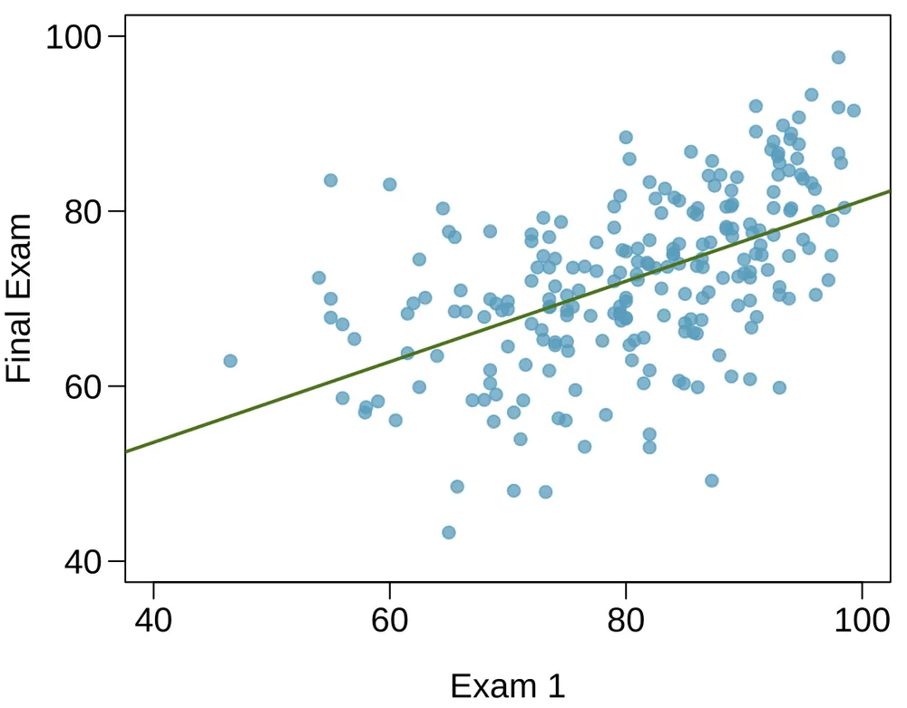
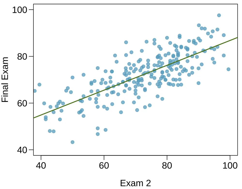
Exams and grades. The two scatterplots below show the relationship between final and mid-semester exam grades recorded during several years for a Statistics course at a university.
Based on these graphs, which of the two exams has the strongest correlation with the final exam grade? Explain.
Can you think of a reason why the correlation between the exam you chose in part (a) and the final exam is higher?
Exercise 8.6
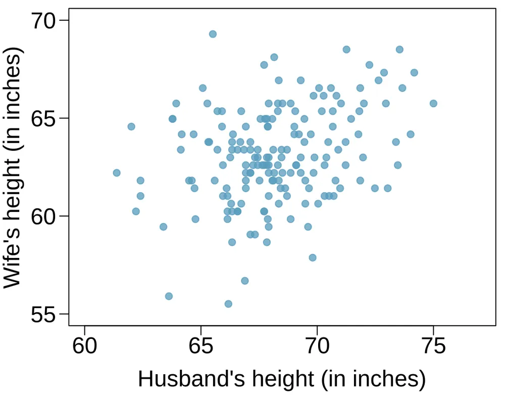
Husbands and wives, Part I. The Great Britain Office of Population Census and Surveys once collected data on a random sample of 170 married couples in Britain, recording the age (in years) and heights (converted here to inches) of the husbands and wives.5 The scatterplot on the left shows the wife’s age plotted against her husband’s age, and the plot on the right shows wife’s height plotted against husband’s height.
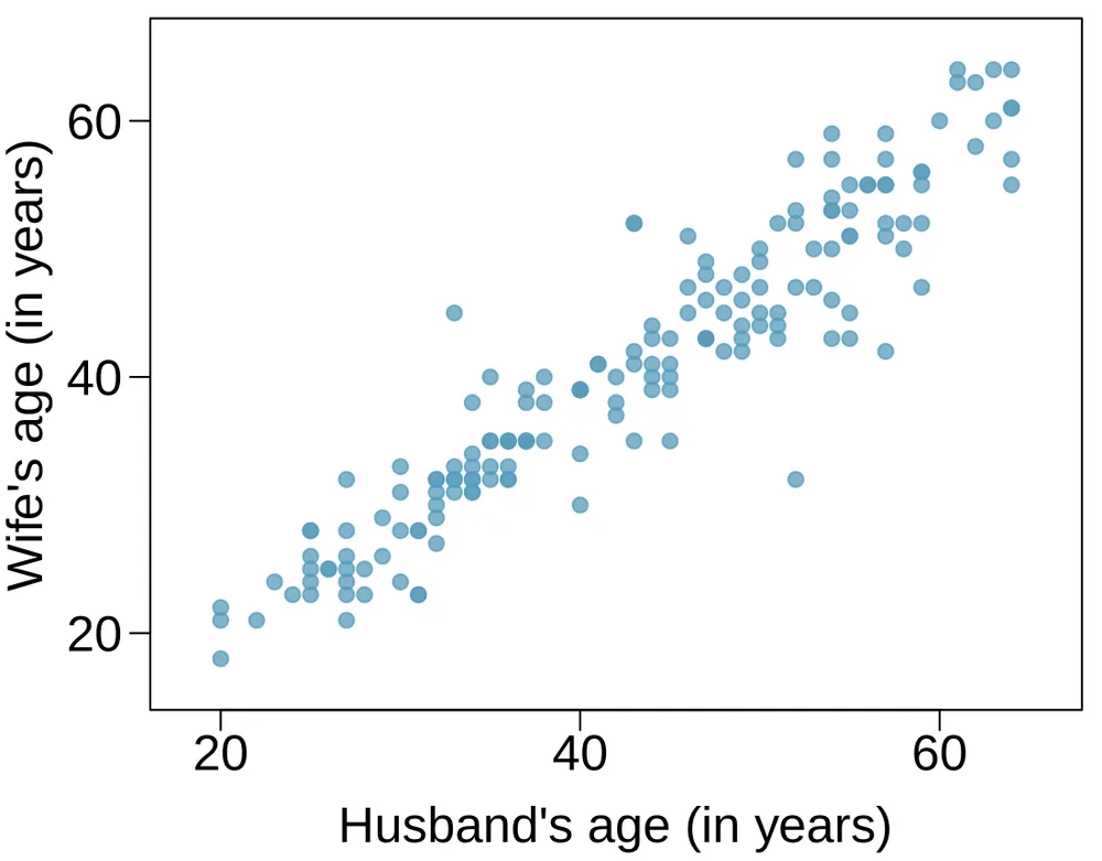
Describe the relationship between husbands’ and wives’ ages.
Describe the relationship between husbands’ and wives’ heights.
Which plot shows a stronger correlation? Explain your reasoning.
Data on heights were originally collected in centimeters, and then converted to inches. Does this conversion affect the correlation between husbands’ and wives’ heights?
Exercise 8.7
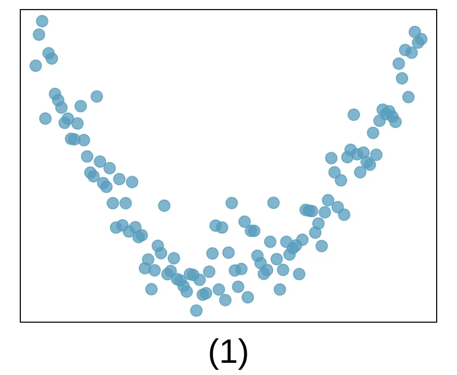
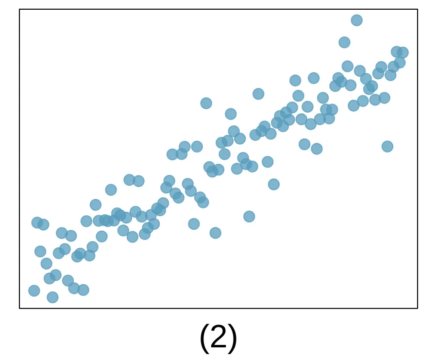
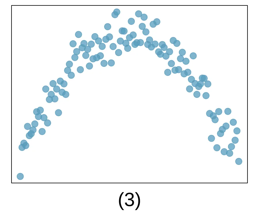
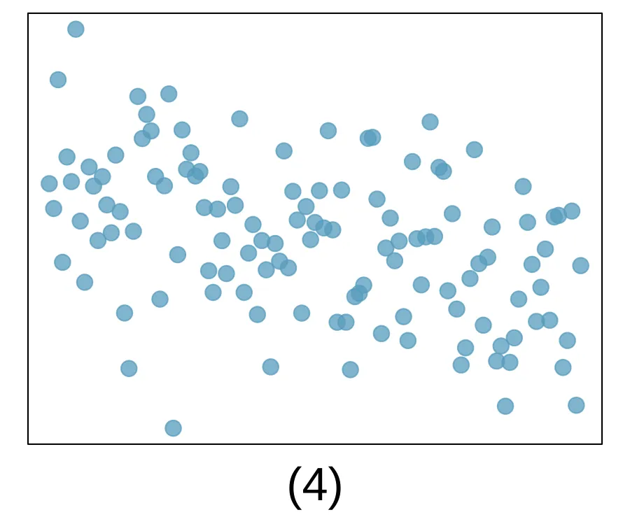
Match the correlation, Part I. Match each correlation to the corresponding scatterplot.
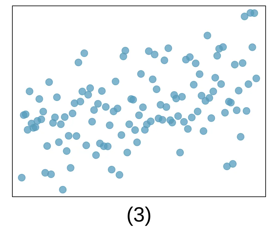
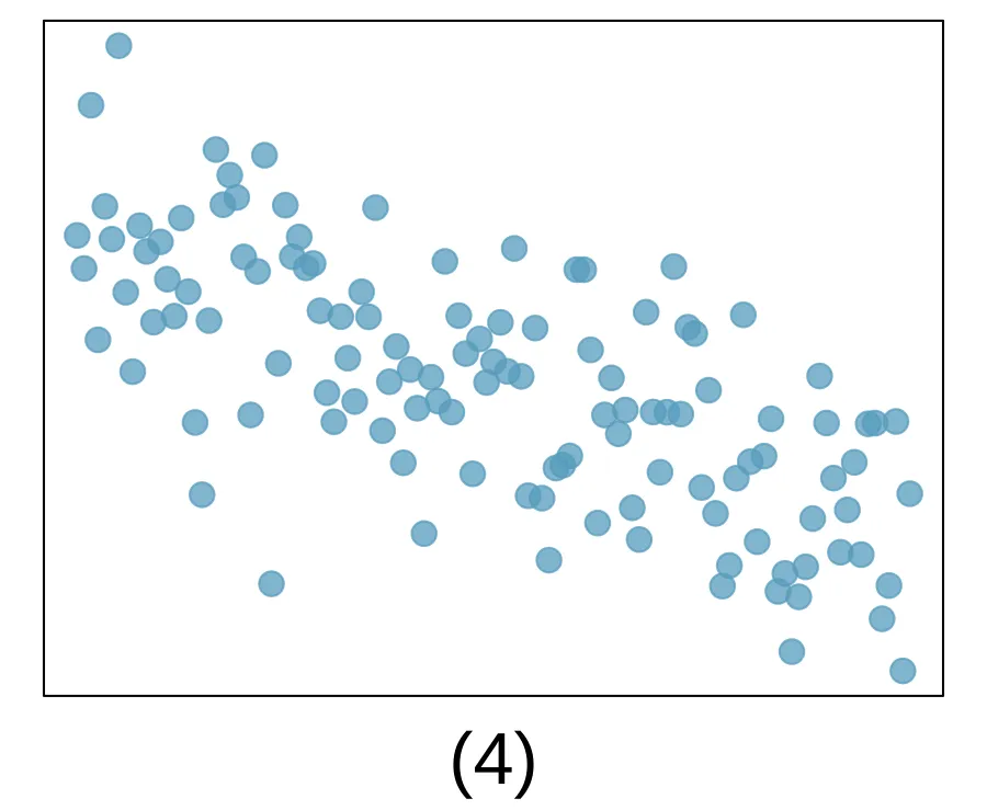
Exercise 8.8
Match the correlation, Part II. Match each correlation to the corresponding scatterplot.
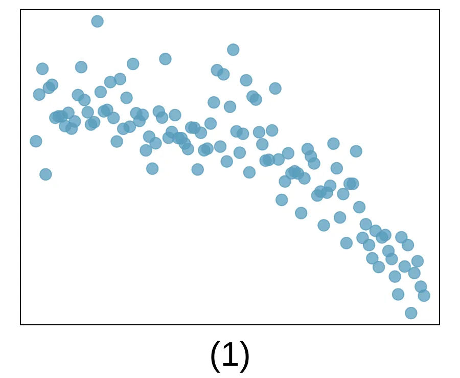
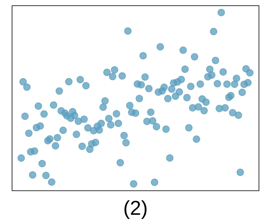
Exercise 8.9
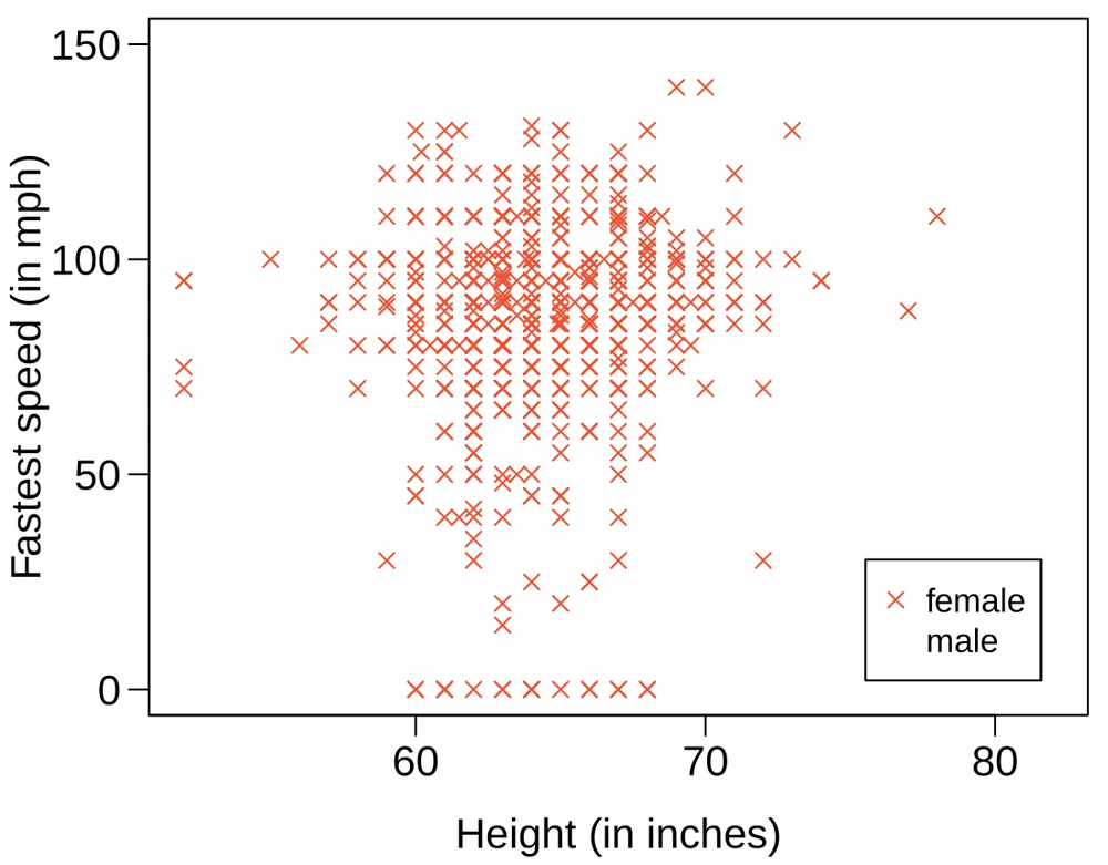
Speed and height. 1,302 UCLA students were asked to fill out a survey where they were asked about their height, fastest speed they have ever driven, and gender. The scatterplot on the left displays the relationship between height and fastest speed, and the scatterplot on the right displays the breakdown by gender in this relationship.
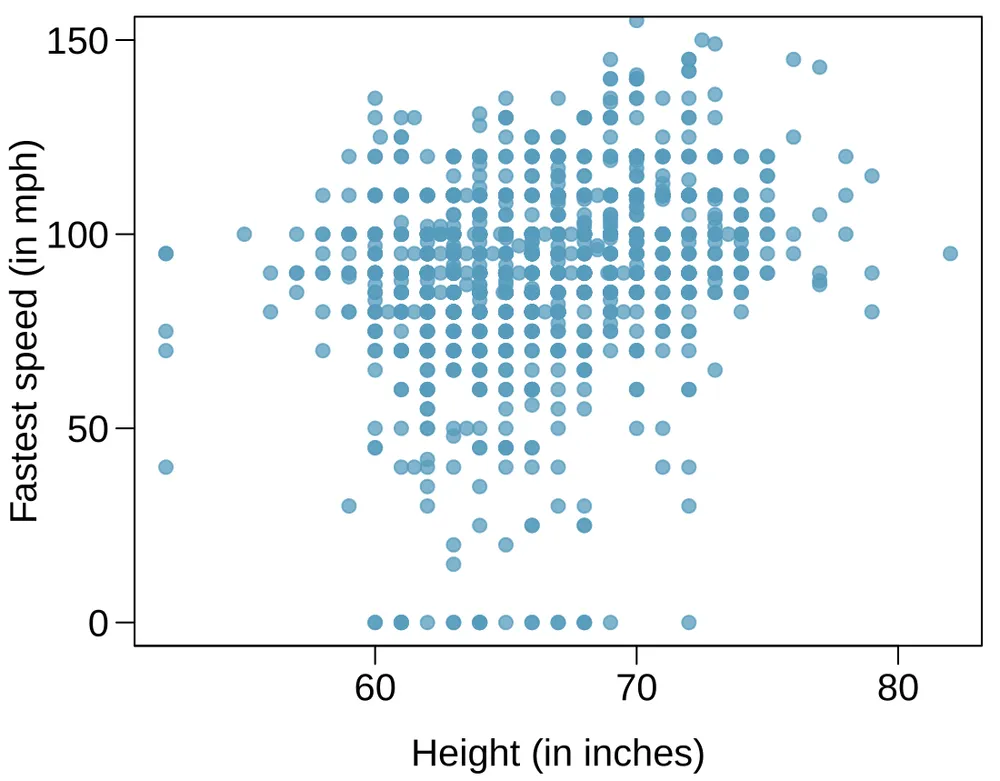
Describe the relationship between height and fastest speed.
Why do you think these variables are positively associated?
What role does gender play in the relationship between height and fastest driving speed?
Exercise 8.10
Guess the correlation. Eduardo and Rosie are both collecting data on number of rainy days in a year and the total rainfall for the year. Eduardo records rainfall in inches and Rosie in centimeters. How will their correlation coefficients compare?
Exercise 8.11
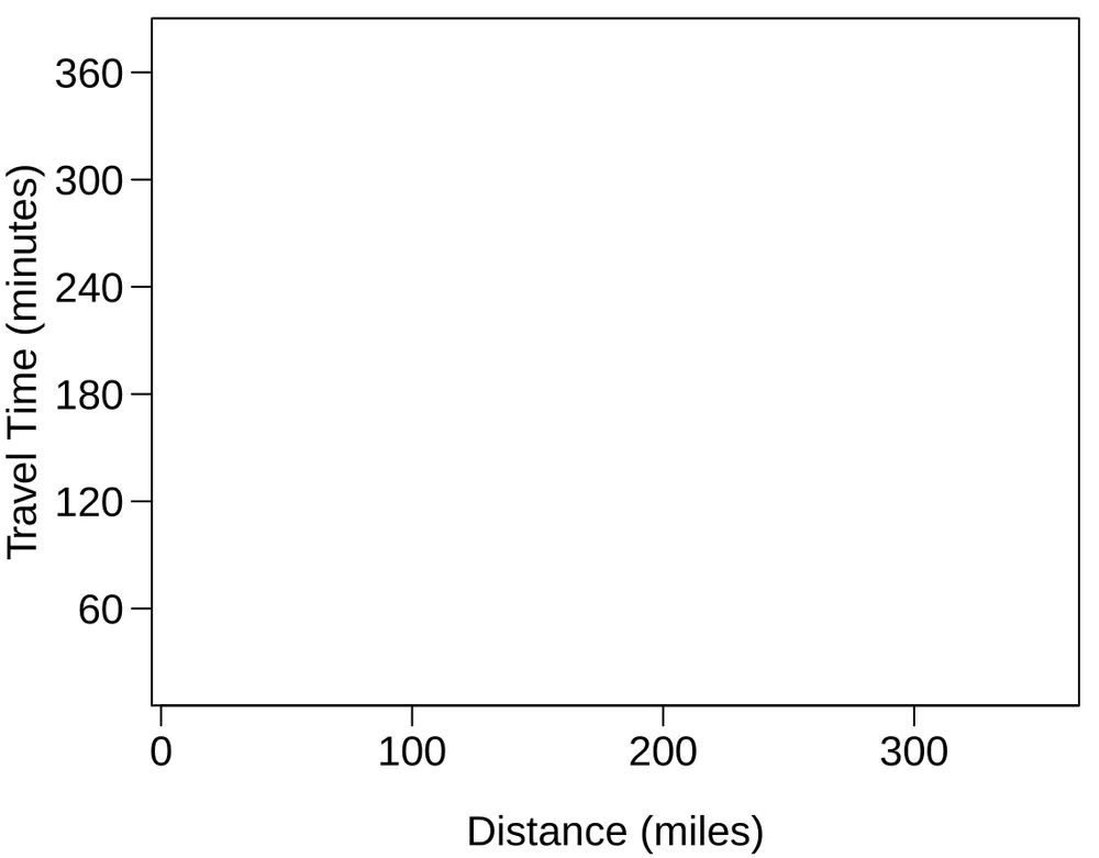
The Coast Starlight, Part I. The Coast Starlight Amtrak train runs from Seattle to Los Angeles. The scatterplot below displays the distance between each stop (in miles) and the amount of time it takes to travel from one stop to another (in minutes).
Describe the relationship between distance and travel time.
How would the relationship change if travel time was instead measured in hours, and distance was instead measured in kilometers?
The correlation between travel time (in miles) and distance (in minutes) is . Suppose we had instead measured travel time in hours and measured distance in kilometers (km). What would be the correlation in these different units?
Exercise 8.12
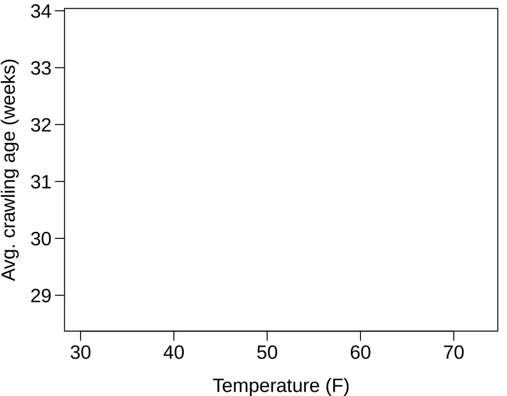
Crawling babies, Part I. A study conducted at the University of Denver investigated whether babies take longer to learn to crawl in cold months, when they are often bundled in clothes that restrict their movement, than in warmer months. 6 Infants born during the study year were split into twelve groups, one for each birth month. We consider the average crawling age of babies in each group against the average temperature when the babies are six months old (that’s when babies often begin trying to crawl). Temperature is measured in degrees Fahrenheit (^F) and age is measured in weeks.
Describe the relationship between temperature and crawling age.
How would the relationship change if temperature was measured in degrees Celsius (^C) and age was measured in months?
The correlation between temperature in ^F and age in weeks was . If we converted the temperature to ^C and age to months, what would the correlation be?
Exercise 8.13
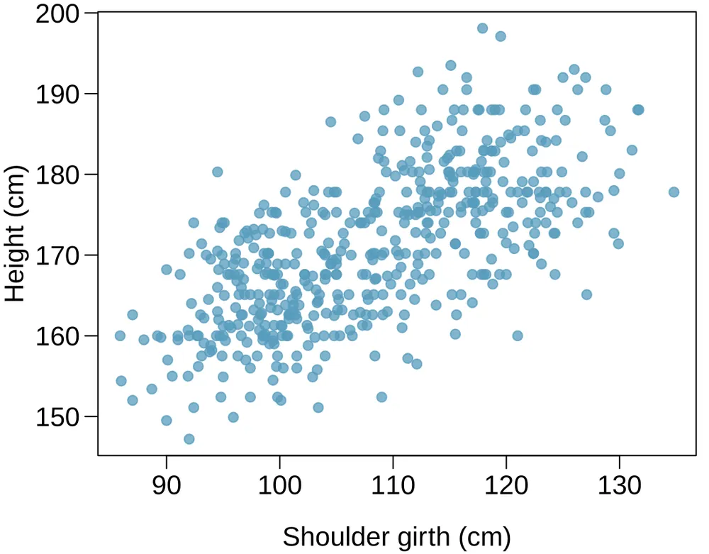
Body measurements, Part I. Researchers studying anthropometry collected body girth measurements and skeletal diameter measurements, as well as age, weight, height and gender for 507 physically active individuals.7 The scatterplot below shows the relationship between height and shoulder girth (over deltoid muscles), both measured in centimeters.
Describe the relationship between shoulder girth and height.
How would the relationship change if shoulder girth was measured in inches while the units of height remained in centimeters?
Exercise 8.14
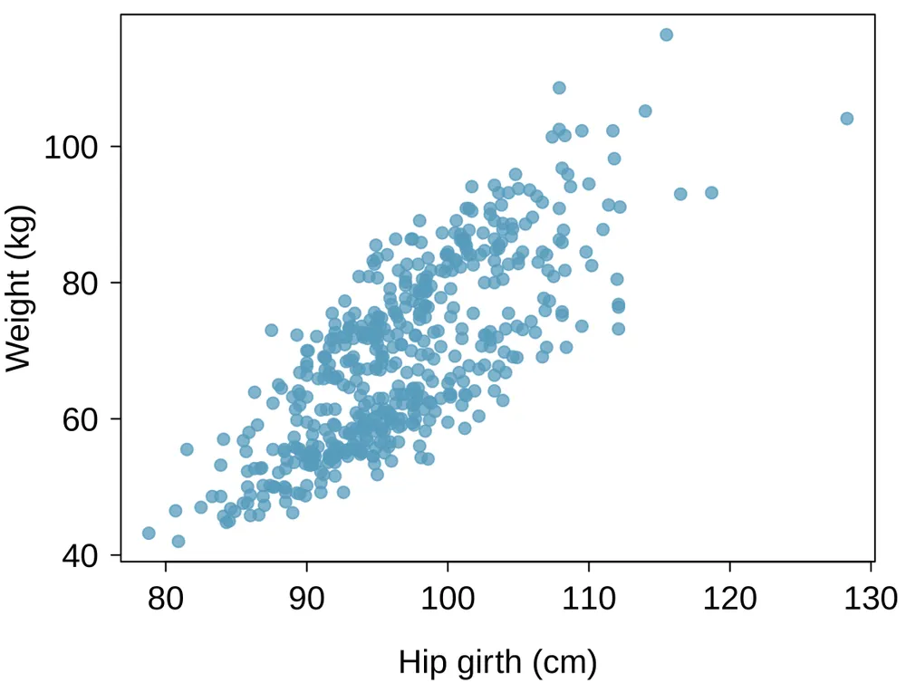
Body measurements, Part II. The scatterplot below shows the relationship between weight measured in kilograms and hip girth measured in centimeters from the data described in Exercise 8.13.
Describe the relationship between hip girth and weight.
How would the relationship change if weight was measured in pounds while the units for hip girth remained in centimeters?
Exercise 8.15
Correlation, Part I. What would be the correlation between the ages of husbands and wives if men always married woman who were
3 years younger than themselves?
2 years older than themselves?
half as old as themselves?
Exercise 8.16
Correlation, Part II. What would be the correlation between the annual salaries of males and females at a company if for a certain type of position men always made
$5,000 more than women?
25% more than women?
15% less than women?
Notes
If a model underestimates an observation, then the model estimate is below the actual. The residual, which is the actual observation value minus the model estimate, must then be positive. The opposite is true when the model overestimates the observation: the residual is negative. ↩
() First compute the predicted value based on the model: Then the residual is given by This was close to the earlier estimate of 7.
() . , close to the estimate of -4. ↩
Formally, we can compute the correlation for observations , , ..., using the formula where , , , and are the sample means and standard deviations for each variable. ↩
We’ll leave it to you to draw the lines. In general, the lines you draw should be close to most points and reflect overall trends in the data. ↩
Hand, D.J. A handbook of small data sets. Chapman & Hall/CRC. 1994. ↩
Benson, J.B. Season of birth and onset of locomotion: Theoretical and methodological implications. Infant behavior and development. 1993. ↩
Heinz, G. et al. Exploring relationships in body dimensions. Journal of Statistics Education. 2003. ↩