Motivating Questions
- What geometric condition enables us to optimize a function subject to a constraint given by where is a constant?
- How can we exploit this geometric condition to find the extreme values of a function subject to a constraint?
We previously considered how to find the extreme values of functions on both unrestricted domains and on closed, bounded domains. Other types of optimization problems involve maximizing or minimizing a quantity subject to an external constraint. In these cases the extreme values frequently won't occur at the points where the gradient is zero, but rather at other points that satisfy an important geometric condition. These problems are often called constrained optimization problems and can be solved with the method of Lagrange Multipliers, which we study in this section.
Preview Activity
According to U.S. postal regulations, the girth plus the length of a parcel sent by mail may not exceed 108 inches, where by “girth” we mean the perimeter of the smallest end. Our goal is to find the largest possible volume of a rectangular parcel with a square end that can be sent by mail. (We solved this applied optimization problem in single variable Active Calculus, so it may look familiar. We take a different approach in this section, and this approach allows us to view most applied optimization problems from single variable calculus as constrained optimization problems, as well as provide us tools to solve a greater variety of optimization problems.) If we let be the length of the side of one square end of the package and the length of the package, then we want to maximize the volume of the box subject to the constraint that the girth () plus the length () is as large as possible, or The equation is thus an external constraint on the variables.
- The constraint equation involves the function that is given by
Explain why the constraint is a contour of and is therefore a two-dimensional curve.
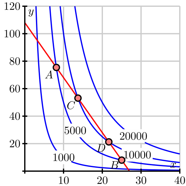
-
Figure . Contours of and the constraint equation - Figure shows the graph of the constraint equation along with a few contours of the volume function Since our goal is to find the maximum value of subject to the constraint we want to find the point on our constraint curve that intersects the contours of at which has its largest value.
- Points and in Figure lie on a contour of and on the constraint equation Explain why neither nor provides a maximum value of that satisfies the constraint.
- Points and in Figure lie on a contour of and on the constraint equation Explain why neither nor provides a maximum value of that satisfies the constraint.
- Based on your responses to parts i. and ii., draw the contour of on which you believe will achieve a maximum value subject to the constraint Explain why you drew the contour you did.
- Recall that is a contour of the function and that the gradient of a function is always orthogonal to its contours. With this in mind, how should and be related at the optimal point? Explain.
Constrained Optimization and Lagrange Multipliers
In Preview Activity , we considered an optimization problem where there is an external constraint on the variables, namely that the girth plus the length of the package cannot exceed 108 inches. We saw that we can create a function from the constraint, specifically The constraint equation is then just a contour of where is a constant (in our case 108). Figure illustrates that the volume function is maximized, subject to the constraint when the graph of is tangent to a contour of Moreover, the value of on this contour is the sought maximum value.
To find this point where the graph of the constraint is tangent to a contour of recall that is perpendicular to the contours of and is perpendicular to the contour of At such a point, the vectors and are parallel, and thus we need to determine the points where this occurs. Recall that two vectors are parallel if one is a nonzero scalar multiple of the other, so we therefore look for values of a parameter that make
The constant is called a Lagrange multiplier.
To find the values of that satisfy Equation \ref{eq_10_8_Lagrange_ex1} for the volume function in Preview Activity , we calculate both and Observe that
and thus we need a value of so that
Equating components in the most recent equation and incorporating the original constraint, we have three equations
in the three unknowns and First, note that if then Equation \ref{eq_10_8_lag_ex2} shows that From this, Equation \ref{eq_10_8_lag_ex3} tells us that So the point is a point we need to consider. Next, provided that (from which it follows that by Equation \ref{eq_10_8_lag_ex2}, we may divide both sides of Equation \ref{eq_10_8_lag_ex1} by the corresponding sides of Equation \ref{eq_10_8_lag_ex2} to eliminate and thus find that
Substituting into Equation \ref{eq_10_8_lag_ex3} gives us
or
Thus we have and as another point to consider. So the points at which the gradients of and are parallel, and thus at which may have a maximum or minimum subject to the constraint, are and By evaluating the function at these points, we see that we maximize the volume when the length of the square end of the box is 18 inches and the length is 36 inches, for a maximum volume of cubic inches. Since we obtain a minimum value at this point.
We summarize the process of Lagrange multipliers as follows.
The method of Lagrange multipliers
The general technique for optimizing a function subject to a constraint is to solve the system and for and We then evaluate the function at each point that results from a solution to the system in order to find the optimum values of subject to the constraint.
Activity
A cylindrical soda can holds about 355 cc of liquid. In this activity, we want to find the dimensions of such a can that will minimize the surface area. For the sake of simplicity, assume the can is a perfect cylinder.
- What are the variables in this problem? Based on the context, what restriction(s), if any, are there on these variables?
- What quantity do we want to optimize in this problem? What equation describes the constraint? (You need to decide which of these functions plays the role of and which plays the role of in our discussion of Lagrange multipliers.)
- Find and the values of your variables that satisfy Equation \ref{eq_10_8_Lagrange_ex1} in the context of this problem.
- Determine the dimensions of the pop can that give the desired solution to this constrained optimization problem.
The method of Lagrange multipliers also works for functions of more than two variables.
Activity
Use the method of Lagrange multipliers to find the dimensions of the least expensive packing crate with a volume of 240 cubic feet when the material for the top costs $2 per square foot, the bottom is $3 per square foot and the sides are $1.50 per square foot.
The method of Lagrange multipliers also works for functions of three variables. That is, if we have a function that we want to optimize subject to a constraint the optimal point lies on the level surface defined by the constraint As we did in Preview Activity , we can argue that the optimal value occurs at the level surface that is tangent to Thus, the gradients of and are parallel at this optimal point. So, just as in the two variable case, we can optimize subject to the constraint by finding all points that satisfy and
Summary
- The extrema of a function subject to a constraint occur at points for which the contour of is tangent to the curve that represents the constraint equation. This occurs when
- We use the condition to generate a system of equations, together with the constraint that may be solved for and Once we have all the solutions, we evaluate at each of the points to determine the extrema.