Motivating Questions
- The partial derivatives of a function tell us the rate of change of in the direction of the coordinate axes. How can we measure the rate of change of in other directions?
- What is the gradient of a function and what does it tell us?
The partial derivatives of a function tell us the instantaneous rate at which the function changes as we hold all but one independent variable constant and allow the remaining independent variable to change. It is natural to wonder how we can measure the rate at which a function changes in directions other than parallel to a coordinate axes. In what follows, we investigate this question, and see how the rate of change in any given direction is connected to the rates of change given by the standard partial derivatives.
Preview Activity
Let's consider the function defined by
and suppose that measures the temperature, in degrees Celsius, at a given point in the plane, where and are measured in feet. Assume that the positive -axis points due east, while the positive -axis points due north. A contour plot of is shown in Figure .
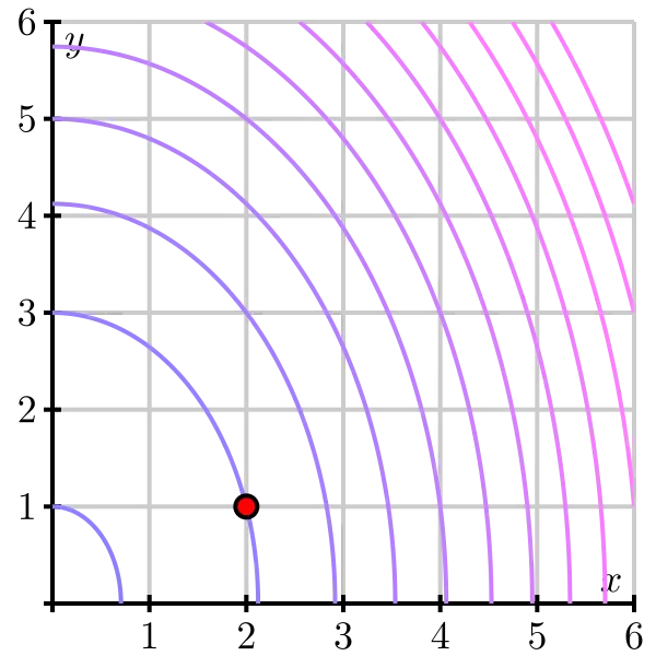
- Suppose that a person is walking due east, and thus parallel to the -axis. At what instantaneous rate is the temperature changing with respect to at the moment the walker passes the point What are the units on this rate of change?
- Next, determine the instantaneous rate of change of temperature with respect to distance at the point if the person is instead walking due north. Again, include units on your result.
- Now, rather than walking due east or due north, let's suppose that the person is walking with velocity given by the vector where time is measured in seconds. Note that the person's speed is thus feet per second. Find parametric equations for the person's path; that is, parameterize the line through using the direction vector Let denote the -coordinate of the line, and its -coordinate. Make sure your parameterization places the walker at the point when
- With the parameterization in (c), we can now view the temperature as not only a function of and but also of time, Hence, use the chain rule to determine the value of What are the units on your answer? What is the practical meaning of this result?
Directional Derivatives
Given a function the partial derivative measures the instantaneous rate of change of as only the variable changes; likewise, measures the rate of change of at as only changes. Note particularly that is measured in “units of per unit of change in ” and that the units on are similar.
In Preview Activity , we saw how we could measure the rate of change of in a situation where both and were changing; in that activity, however, we found that this rate of change was measured in “units of per unit of time.” In a given unit of time, we may move more than one unit of distance. In fact, in Preview Activity , in each unit increase in time we move a distance of feet. To generalize the notion of partial derivatives to any direction of our choice, we instead want to have a rate of change whose units are “units of per unit of distance in the given direction.”
In this light, in order to formally define the derivative in a particular direction of motion, we want to represent the change in for a given unit change in the direction of motion. We can represent this unit change in direction with a unit vector, say If we move a distance in the direction of from a fixed point we then arrive at the new point It now follows that the slope of the secant line to the curve on the surface through in the direction of through the points and is
To get the instantaneous rate of change of in the direction we must take the limit of the quantity in Equation \ref{eq_10_6_diff_quot} as Doing so results in the formal definition of the directional derivative.
Definition
Let be given. The derivative of at the point in the direction of the unit vector is denoted and is given by
for those values of and for which the limit exists.
The quantity is called a directional derivative. When we evaluate the directional derivative at a point the result tells us the instantaneous rate at which changes at per unit increase in the direction of the vector In addition, the quantity tells us the slope of the line tangent to the surface in the direction of at the point
Computing the Directional Derivative
In a similar way to how we developed shortcut rules for standard derivatives in single variable calculus, and for partial derivatives in multivariable calculus, we can also find a way to evaluate directional derivatives without resorting to the limit definition found in Equation \ref{E_DirDerDef}. We do so using a very similar approach to our work in Preview Activity .
Suppose we consider the situation where we are interested in the instantaneous rate of change of at a point in the direction where is a unit vector. The variables and are therefore changing according to the parameterization
Observe that and for all values of Since is a unit vector, it follows that a point moving along this line moves one unit of distance per one unit of time; that is, each single unit of time corresponds to movement of a single unit of distance in that direction. This observation allows us to use the Chain Rule to calculate the directional derivative, which measures the instantaneous rate of change of with respect to change in the direction
In particular, by the Chain Rule, it follows that
This now allows us to compute the directional derivative at an arbitrary point according to the following formula.
Calculating a directional derivative
Given a differentiable function and a unit vector we may compute by
Note well: To use Equation \ref{eq_10_6_DD}, we must have a unit vector in the direction of motion. In the event that we have a direction prescribed by a non-unit vector, we must first scale the vector to have length 1.
Activity
Let
- Determine and
- Use Equation \ref{eq_10_6_DD} to determine and What familiar function is What familiar function is (Recall that is the unit vector in the positive -direction and is the unit vector in the positive -direction.)
- Use Equation \ref{eq_10_6_DD} to find the derivative of in the direction of the vector at the point Remember that a unit direction vector is needed.
The Gradient
Via the Chain Rule, we have seen that for a given function its instantaneous rate of change in the direction of a unit vector is given by
Recalling that the dot product of two vectors and is computed by
we see that we may recast Equation \ref{E_DDrevisited} in a way that has geometric meaning. In particular, we see that is the dot product of the vector and the vector
We call this vector formed by the partial derivatives of the gradient of and denote it
We read as “the gradient of ” “grad ” or “del ”. 1 Notice that varies from point to point, and also provides an alternate formulation of the directional derivative.
The directional derivative and the gradient
Given a differentiable function and a unit vector we may compute by
In the following activity, we investigate some of what the gradient tells us about the behavior of a function
Activity
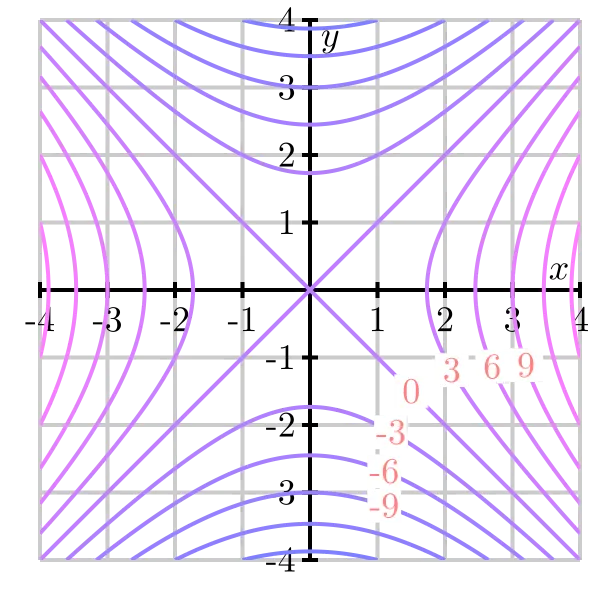
Let's consider the function defined by Some contours for this function are shown in Figure .
- Find the gradient
- For each of the following points evaluate the gradient and sketch the gradient vector with its tail at Some of the vectors are too long to fit onto the plot, but we'd like to draw them to scale; to do so, scale each vector by a factor of 1/4.
- What do you notice about the relationship between the gradient at and the contour passing through that point?
- Does increase or decrease in the direction of Provide a justification for your response.
As a vector, defines a direction and a length. As we will soon see, both of these convey important information about the behavior of near
The Direction of the Gradient
Remember that the dot product also conveys information about the angle between the two vectors. If is the angle between and (where is a unit vector), then we also have that
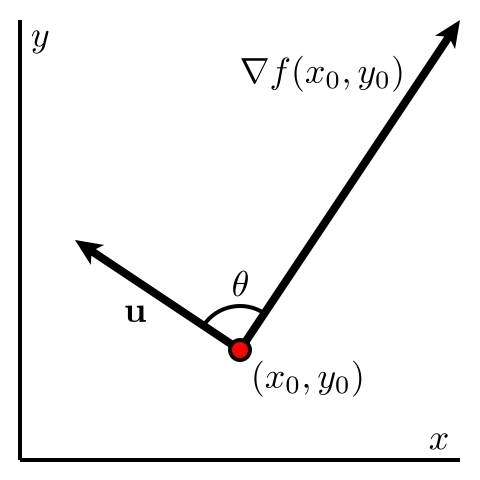
In particular, when is a right angle, as shown on the left of Figure , then because Since the value of the directional derivative is 0, this means that is unchanging in this direction, and hence must be tangent to the contour of that passes through In other words, is orthogonal to the contour through This shows that the gradient vector at a given point is always perpendicular to the contour passing through the point, confirming that what we saw in part (c) of Activity holds in general.
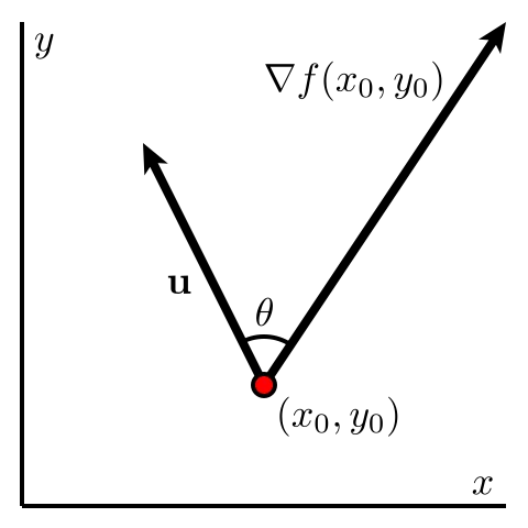
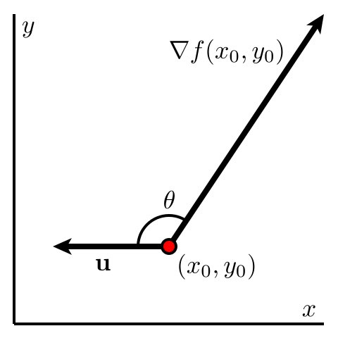
Moreover, when is an acute angle, it follows that so since
and therefore as shown in the middle image in Figure . This means that is increasing in any direction where is acute. In a similar way, when is an obtuse angle, then so as seen on the right in Figure . This means that is decreasing in any direction for which is obtuse.
Finally, as we can see in the following activity, we may also use the gradient to determine the directions in which the function is increasing and decreasing most rapidly.
Activity
In this activity we investigate how the gradient is related to the directions of greatest increase and decrease of a function. Let be a differentiable function and a unit vector.
- Let be the angle between and Use the relationship between the dot product and the angle between two vectors to explain why
- At the point the only quantity in Equation \ref{eq_10_6_DD_grad2} that can change is (which determines the direction of travel). Explain why makes the quantity
as large as possible.
- When in what direction does the unit vector point relative to Why? What does this tell us about the direction of greatest increase of at the point
- In what direction, relative to does decrease most rapidly at the point
- State the unit vectors and (in terms of ) that provide the directions of greatest increase and decrease for the function at the point What important assumption must we make regarding in order for these vectors to exist?
The Length of the Gradient
Having established in Activity that the direction in which a function increases most rapidly at a point is the unit vector in the direction of the gradient, (that is, provided that ), it is also natural to ask, “in the direction of greatest increase for at what is the value of the rate of increase?” In this situation, we are asking for the value of where
Using the now familiar way to compute the directional derivative, we see that
Next, we recall two important facts about the dot product: (i) for any scalar and (ii) Applying these properties to the most recent equation involving the directional derivative, we find that
Finally, since is a nonzero vector, its length is a nonzero scalar, and thus we can simplify the preceding equation to establish that
We summarize our most recent work by stating two important facts about the gradient.
Important facts about the gradient
Let be a differentiable function and a point for which Then points in the direction of greatest increase of at and the instantaneous rate of change of in that direction is the length of the gradient vector. That is, if then is a unit vector in the direction of greatest increase of at and
Activity
Consider the function defined by
a. Find the gradient and sketch it on Figure .
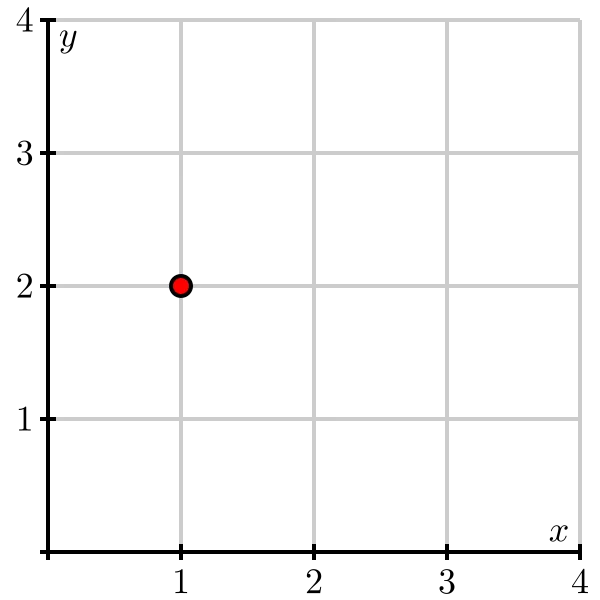
b. Sketch the unit vector on Figure with its tail at Now find the directional derivative
c. What is the slope of the graph of in the direction What does the sign of the directional derivative tell you?
d. Consider the vector and sketch on Figure with its tail at Find a unit vector pointing in the same direction of Without computing what do you know about the sign of this directional derivative? Now verify your observation by computing
e. In which direction (that is, for what unit vector ) is the greatest? What is the slope of the graph in this direction?
f. Corresponding, in which direction is least? What is the slope of the graph in this direction?
g. Sketch two unit vectors for which and then find component representations of these vectors.
h. Suppose you are standing at the point In which direction should you move to cause to increase as rapidly as possible? At what rate does increase in this direction?
Applications
The gradient finds many natural applications. For example, situations often arise — for instance, constructing a road through the mountains or planning the flow of water across a landscape — where we are interested in knowing the direction in which a function is increasing or decreasing most rapidly.
For example, consider a two-dimensional version of how a heat-seeking missile might work.(This application is borrowed from United States Air Force Academy Department of Mathematical Sciences.) Suppose that the temperature surrounding a fighter jet can be modeled by the function defined by
where is a point in the plane of the fighter jet and is measured in degrees Celsius. Some contours and gradients are shown on the left in Figure .
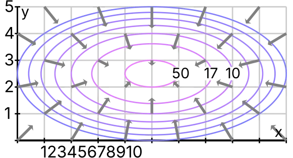
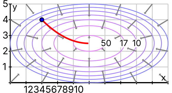
A heat-seeking missile will always travel in the direction in which the temperature increases most rapidly; that is, it will always travel in the direction of the gradient If a missile is fired from the point then its path will be that shown on the right in Figure .
In the final activity of this section, we consider several questions related to this context of a heat-seeking missile, and foreshadow some upcoming work in Section 10.7.
Activity
- The temperature has its maximum value at the fighter jet's location. State the fighter jet's location and explain how Figure tells you this.
- Determine at the fighter jet's location and give a justification for your response.
- Suppose that a different function has a local maximum value at Sketch the behavior of some possible contours near this point. What is (Hint: What is the direction of greatest increase in at the local maximum?)
- Suppose that a function has a local minimum value at Sketch the behavior of some possible contours near this point. What is
- If a function has a local minimum at what is the direction of greatest increase of at
Summary
- The directional derivative of at the point in the direction of the unit vector is
for those values of and for which the limit exists. In addition, measures the slope of the graph of when we move in the direction Alternatively, measures the instantaneous rate of change of in the direction at
- The gradient of a function at a point is the vector
- The directional derivative in the direction may be computed by
- At any point where the gradient is nonzero, gradient is orthogonal to the contour through that point and points in the direction in which increases most rapidly; moreover, the slope of in this direction equals the length of the gradient Similarly, the opposite of the gradient points in the direction of greatest decrease, and that rate of decrease is the opposite of the length of the gradient.