Motivating Questions

What is the Chain Rule and how do we use it to find a derivative?
How can we use a tree diagram to guide us in applying the Chain Rule?

In single-variable calculus, we encountered situations in which some quantity $z$ depends on $y$ and, in turn, $y$ depends on $x\text{.}$ A change in $x$ produces a change in $y\text{,}$ which consequently produces a change in $z\text{.}$ Using the language of differentials that we saw in the previous section, these changes are naturally related by

$dz = \frac{dz}{dy}~dy \ \mbox{and} \ dy = \frac{dy}{dx}~dx.$

In terms of instantaneous rates of change, we then have

dz = \frac{dz}{dy}\frac{dy}{dx}~dx = \frac{dz}{dx}~dx

and thus

\frac{dz}{dx} = \frac{dz}{dy}\frac{dy}{dx}.

This most recent equation we call the Chain Rule.

In the case of a function $f$ of two variables where $z = f(x,y)\text{,}$ it might be that both $x$ and $y$ depend on another variable $t\text{.}$ A change in $t$ then produces changes in both $x$ and $y\text{,}$ which then cause $z$ to change. In this section we will see how to find the change in $z$ that is caused by a change in $t\text{,}$ leading us to multivariable versions of the Chain Rule involving both regular and partial derivatives.

Preview Activity $10.5.1$

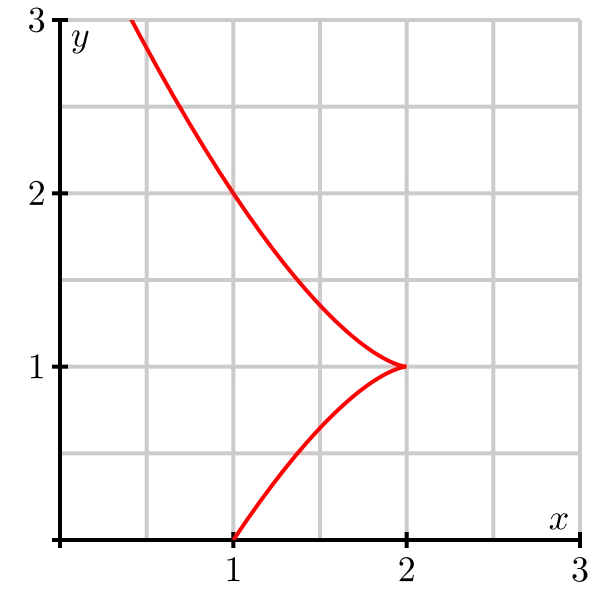
Suppose you are driving around in the $xy$ -plane in such a way that your position $\mathbf{r}(t)$ at time $t$ is given by function

\mathbf{r}(t) = \langle x(t), y(t) \rangle = \langle 2-t^2, t^3 + 1\rangle.

The path taken is shown on the left of Figure $10.5.1$ .

Figure

10.5.1

. Left: Your position in the plane. Right: The corresponding temperature.

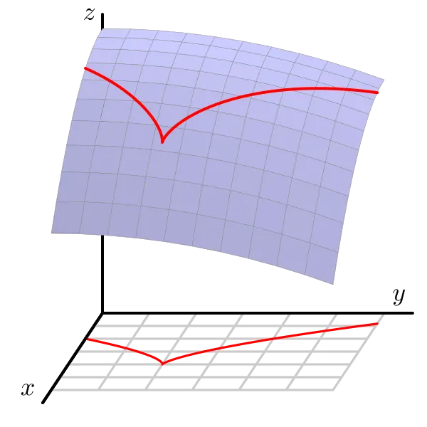
Suppose, furthermore, that the temperature at a point in the plane is given by

T(x,y) = 10 - \frac12x^2 -\frac15y^2,

and note that the surface generated by $T$ is shown on the right of Figure $10.5.1$ . Therefore, as time passes, your position $(x(t), y(t))$ changes, and, as your position changes, the temperature $T(x,y)$ also changes.

The position function $\mathbf r$ provides a parameterization $x = x(t)$ and $y = y(t)$ of the position at time $t\text{.}$ By substituting $x(t)$ for $x$ and $y(t)$ for $y$ in the formula for $T\text{,}$ we can write $T = T(x(t), y(t))$ as a function of $t\text{.}$ Make these substitutions to write $T$ as a function of $t$ and then use the Chain Rule from single variable calculus to find $\frac{dT}{dt}\text{.}$ (Do not do any algebra to simplify the derivative, either before taking the derivative, nor after.)
Now we want to understand how the result from part (a) can be obtained from $T$ as a multivariable function. Recall from the previous section that small changes in $x$ and $y$ produce a change in $T$ that is approximated by
$\Delta T \approx T_x\Delta x + T_y\Delta y.$

The Chain Rule tells us about the instantaneous rate of change of $T\text{,}$ and this can be found as

$\lim_{\Delta t \to 0} \frac{\Delta T}{\Delta t} = \lim_{\Delta t \to 0} \frac{T_x \Delta x + T_y \Delta y}{\Delta t}.$

Use Equation \ref{eq_PA_10_5_1} to explain why the instantaneous rate of change of $T$ that results from a change in $t$ is

$\frac{dT}{dt} = \frac{\partial T}{\partial x} \frac{dx}{dt} + \frac{\partial T}{\partial y} \frac{dy}{dt}.$
Using the original formulas for $T\text{,}$ $x\text{,}$ and $y$ in the problem statement, calculate all of the derivatives in Equation \ref{eq_PA_10_5_2} (with $T_x$ and $T_y$ in terms of $x$ and $y\text{,}$ and $x'$ and $y'$ in terms of $t$ ), and hence write the right-hand side of Equation \ref{eq_PA_10_5_2} in terms of $x\text{,}$ $y\text{,}$ and $t\text{.}$
Compare the results of parts (a) and (c). Write a couple of sentences that identify specifically how each term in (c) relates to a corresponding terms in (a). This connection between parts (a) and (c) provides a multivariable version of the Chain Rule.

As Preview Activity $10.5.1$ suggests, the following version of the Chain Rule holds in general.

Chain Rule

Let $z = f(x,y)\text{,}$ where $f$ is a differentiable function of the independent variables $x$ and $y\text{,}$ and let $x$ and $y$ each be differentiable functions of an independent variable $t\text{.}$ Then

$\frac{dz}{dt} = \frac{\partial z}{\partial x} \frac{dx}{dt} + \frac{\partial z}{\partial y} \frac{dy}{dt}.$

It is important to note the differences among the derivatives in Equation \ref{E_10_5_chain_rule}. Since $z$ is a function of the two variables $x$ and $y\text{,}$ the derivatives in the Chain Rule for $z$ with respect to $x$ and $y$ are partial derivatives. However, since $x = x(t)$ and $y = y(t)$ are functions of the single variable $t\text{,}$ their derivatives are the standard derivatives of functions of one variable. When we compose $z$ with $x(t)$ and $y(t)\text{,}$ we then have $z$ as a function of the single variable $t\text{,}$ making the derivative of $z$ with respect to $t$ a standard derivative from single variable calculus as well.

To understand why this Chain Rule works in general, suppose that some quantity $z$ depends on $x$ and $y$ so that

dz = \frac{\partial z}{\partial x}~dx + \frac{\partial z}{\partial y}~dy.

Next, suppose that $x$ and $y$ each depend on another quantity $t\text{,}$ so that

dx = \frac{dx}{dt}~dt \ \mbox{and} \ dy = \frac{dy}{dt}~dt.

Combining Equations \ref{E_10_5_1} and \ref{E_10_5_2}, we find that

dz = \frac{\partial z}{\partial x}\frac{dx}{dt}~dt + \frac{\partial z}{\partial y}\frac{dy}{dt}~dt = \frac{dz}{dt}~dt,

which is the Chain Rule in this particular context, as expressed in Equation \ref{E_10_5_chain_rule}.

Activity $10.5.2$

In the following questions, we apply the Chain Rule in several different contexts.

Suppose that we have a function $z$ defined by $z(x,y) = x^2+xy^3\text{.}$ In addition, suppose that $x$ and $y$ are restricted to points that move around the plane by following a circle of radius $2$ centered at the origin that is parameterized by
$x(t) = 2\cos(t), \ \mbox{and } \ y(t) = 2\sin(t).$
1. Use the Chain Rule to find the resulting instantaneous rate of change $\frac{dz}{dt}\text{.}$
2. Substitute $x(t)$ for $x$ and $y(t)$ for $y$ in the rule for $z$ to write $z$ in terms of $t$ and calculate $\frac{dz}{dt}$ directly. Compare to the result of part (i.).
Suppose that the temperature on a metal plate is given by the function $T$ with
$T(x,y) = 100-(x^2 + 4y^2),$

where the temperature is measured in degrees Fahrenheit and $x$ and $y$ are each measured in feet.
1. Find $T_x$ and $T_y\text{.}$ What are the units on these partial derivatives?
2. Suppose an ant is walking along the $x$ -axis at the rate of 2 feet per minute toward the origin. When the ant is at the point $(2,0)\text{,}$ what is the instantaneous rate of change in the temperature $dT/dt$ that the ant experiences. Include units on your response.
3. Suppose instead that the ant walks along an ellipse with $x = 6\cos(t)$ and $y = 3\sin(t)\text{,}$ where $t$ is measured in minutes. Find $\frac{dT}{dt}$ at $t = \pi/6\text{,}$ $t=\pi/4\text{,}$ and $t = \pi/3\text{.}$ What does this seem to tell you about the path along which the ant is walking?
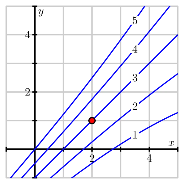
Suppose that you are walking along a surface whose elevation is given by a function $f\text{.}$ Furthermore, suppose that if you consider how your location corresponds to points in the $xy$ -plane, you know that when you pass the point $(2,1)\text{,}$ your velocity vector is $\mathbf v=\langle -1,2\rangle\text{.}$ If some contours of $f$ are as shown in Figure $10.5.2$ , estimate the rate of change $df/dt$ when you pass through $(2,1)\text{.}$

Figure

10.5.2

. Some contours of

f\text{.}

Tree Diagrams

Up to this point, we have applied the Chain Rule to situations where we have a function $z$ of variables $x$ and $y\text{,}$ with both $x$ and $y$ depending on another single quantity $t\text{.}$ We may apply the Chain Rule, however, when $x$ and $y$ each depend on more than one quantity, or when $z$ is a function of more than two variables. It can be challenging to keep track of all the dependencies among the variables, and thus a tree diagram can be a useful tool to organize our work. For example, suppose that $z$ depends on $x$ and $y\text{,}$ and $x$ and $y$ both depend on $t\text{.}$ We may represent these relationships using the tree diagram shown at left Figure $10.5.3$ . We place the dependent variable at the top of the tree and connect it to the variables on which it depends one level below. We then connect each of those variables to the variable on which each depends.

Figure

10.5.3

. A tree diagram illustrating dependencies.

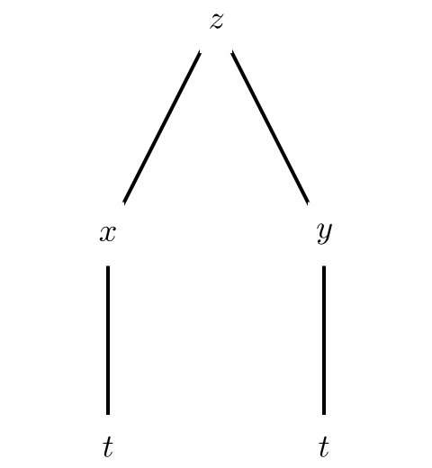
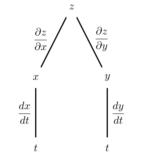
To represent the Chain Rule, we label every edge of the diagram with the appropriate derivative or partial derivative, as seen above in Figure $10.5.3$ . To calculate an overall derivative according to the Chain Rule, we construct the product of the derivatives along all paths connecting the variables and then add all of these products. For example, the diagram above in Figure $10.5.3$ illustrates the Chain Rule

\frac{dz}{dt} = \frac{\partial z}{\partial x}\frac{dx}{dt} + \frac{\partial z}{\partial y}\frac{dy}{dt}.

Activity $10.5.3$

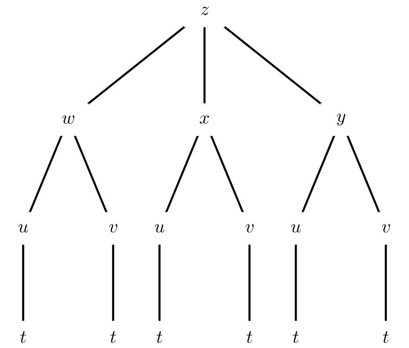
Figure $10.5.4$ shows the tree diagram we construct when (a) $z$ depends on $w\text{,}$ $x\text{,}$ and $y\text{,}$ (b) $w\text{,}$ $x\text{,}$ and $y$ each depend on $u$ and $v\text{,}$ and (c) $u$ and $v$ depend on $t\text{.}$

Figure $10.5.4$ . Three levels of dependencies
1. Label the edges with the appropriate derivatives.
2. Use the Chain Rule to write $\frac{dz}{dt}\text{.}$
Suppose that $z=x^2 - 2xy^2$ and that
$\begin{align*} x& =r\cos(\theta)\\[4pt] y& =r\sin(\theta). \end{align*}$
1. Construct a tree diagram representing the dependencies of $z$ on $x$ and $y$ and $x$ and $y$ on $r$ and $\theta\text{.}$
2. Use the tree diagram to find $\frac{\partial z}{\partial r}\text{.}$
3. Now suppose that $r = 3$ and $\theta=\pi/6\text{.}$ Find the values of $x$ and $y$ that correspond to these given values of $r$ and $\theta\text{,}$ and then use the Chain Rule to find the value of the partial derivative $\frac{\partial z}{\partial \theta}|_{(3,\frac{\pi}{6})}\text{.}$

Summary

The Chain Rule is a tool for differentiating a composite for functions. In its simplest form, it says that if $f(x,y)$ is a function of two variables and $x(t)$ and $y(t)$ depend on $t\text{,}$ then
$\frac{df}{dt} = \frac{\partial f}{\partial x}\frac{dx}{dt} + \frac{\partial f}{\partial y}\frac{dy}{dt}.$
A tree diagram can be used to represent the dependence of variables on other variables. By following the links in the tree diagram, we can form chains of partial derivatives or derivatives that can be combined to give a desired partial derivative.

Build status · Flash Infinity AI™ is a trademark of AI-Flash Inc.. WorldClass is not affiliated with, approved or accredited by any exam board, curriculum provider or university unless a page says so.

10.5: The Chain Rule

Motivating Questions

Preview Activity 10.5.110.5.1

Chain Rule

Activity 10.5.210.5.2

Tree Diagrams

Activity 10.5.310.5.3

Summary

Preview Activity $10.5.1$

Activity $10.5.2$

Activity $10.5.3$