11.5: Double Integrals in Polar Coordinates

Polar Coordinates

The rectangular coordinate system is best suited for graphs and regions that are naturally considered over a rectangular grid. The polar coordinate system is an alternative that offers good options for functions and domains that have more circular characteristics. A point $P$ in rectangular coordinates that is described by an ordered pair $(x,y)\text{,}$ where $x$ is the displacement from $P$ to the $y$-axis and $y$ is the displacement from $P$ to the $x$-axis, as seen in Preview Activity $11.5.1$, can also be described with polar coordinates $(r,\theta)\text{,}$ where $r$ is the distance from $P$ to the origin and $\theta$ is the angle formed by the line segment $\overline{OP}$ and the positive $x$-axis, as shown at left in Figure $11.5.1$.

 

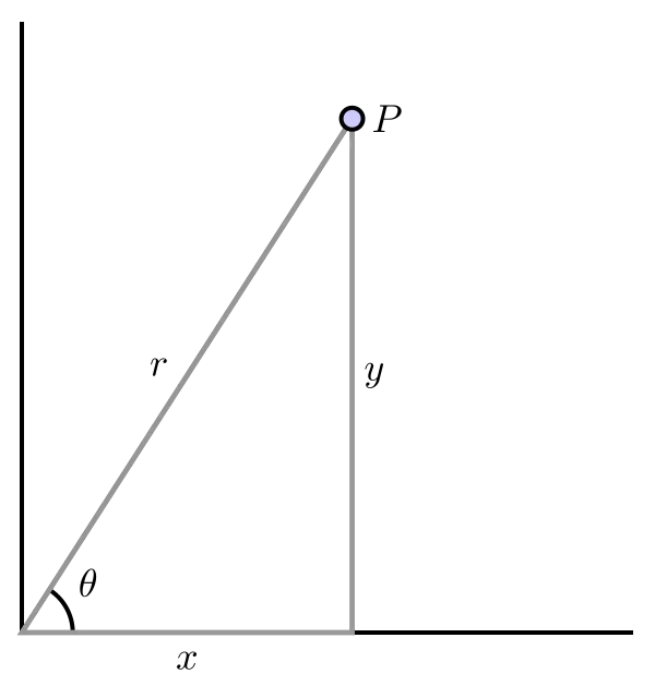
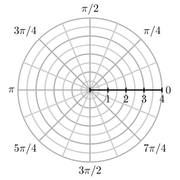
Trigonometry and the Pythagorean Theorem allow for straightforward conversion from rectangular to polar, and vice versa.

Converting between rectangular and polar coordinates

• If we are given the rectangular coordinates $(x,y)$ of a point $P\text{,}$ then the polar coordinates $(r,\theta)$ of $P$ satisfy
  $$r = \sqrt{x^2+y^2} \ \ \ \ \ \text{ and } \ \ \ \ \ \tan(\theta) = \frac{y}{x}, \text{ assuming } x \neq 0.$$
• If we are given the polar coordinates $(r,\theta)$ of a point $P\text{,}$ then the rectangular coordinates $(x,y)$ of $P$ satisfy
  $$x = r\cos(\theta) \ \ \ \ \ \text{ and } \ \ \ \ \ y = r\sin(\theta).$$

Note: The angle $\theta$ in the polar coordinates of a point is not unique. We could replace $\theta$ with $\theta + 2 \pi$ and still be at the same terminal point. In addition, the sign of $\tan(\theta)$ does not uniquely determine the quadrant in which $\theta$ lies, so we have to determine the value of $\theta$ from the location of the point. In other words, more care has to be paid when using polar coordinates than rectangular coordinates.

We can draw graphs of curves in polar coordinates in a similar way to how we do in rectangular coordinates. However, when plotting in polar coordinates, we use a grid that considers changes in angles and changes in distance from the origin. In particular, the angles $\theta$ and distances $r$ partition the plane into small wedges as shown at right in Figure $11.5.1$.

Activity $11.5.2$

Most polar graphing devices can plot curves in polar coordinates of the form $r = f(\theta)\text{.}$ Use such a device to complete this activity.

1. Before plotting the polar curve $r=1$ (where $\theta$ can have any value), think about what shape it should have, in light of how $r$ is connected to $x$ and $y\text{.}$ Then use appropriate technology to draw the graph and test your intuition.
2. The equation $\theta = 1$ does not define $r$ as a function of $\theta\text{,}$ so we can't graph this equation on many polar plotters. What do you think the graph of the polar curve $\theta = 1$ looks like? Why?
3. Before plotting the polar curve $r = \theta\text{,}$ what do you think the graph looks like? Why? Use technology to plot the curve and compare your intuition.
4. What does the region defined by $1 \leq r \leq 3$ (where $\theta$ can have any value) look like? (Hint: Compare to your response from part (a).)
5. What does the region defined by $1 \leq r \leq 3$ and $\pi/4 \leq \theta \leq \pi/2$ look like?
6. Consider the curve $r = \sin(\theta)\text{.}$ For some values of $\theta$ we will have $r \lt 0\text{.}$ In these situations, we plot the point $(r,\theta)$ as $(|r|, \theta+\pi)$ (in other words, when $r \lt 0\text{,}$ we reflect the point through the origin). With that in mind, what do you think the graph of $r = \sin(\theta)$ looks like? Plot this curve using technology and compare to your intuition.

Integrating in Polar Coordinates

Consider the double integral

where $D$ is the unit disk. While we cannot directly evaluate this integral in rectangular coordinates, a change to polar coordinates will convert it to one we can easily evaluate.

We have seen how to evaluate a double integral $\displaystyle \iint_D f(x,y) \, dA$ as an iterated integral of the form

in rectangular coordinates, because we know that $dA = dy \, dx$ in rectangular coordinates. To make the change to polar coordinates, we not only need to represent the variables $x$ and $y$ in polar coordinates, but we also must understand how to write the area element, $dA\text{,}$ in polar coordinates. That is, we must determine how the area element $dA$ can be written in terms of $dr$ and $d\theta$ in the context of polar coordinates. We address this question in the following activity.

 

Activity $11.5.3$

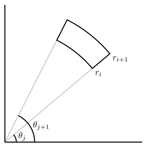
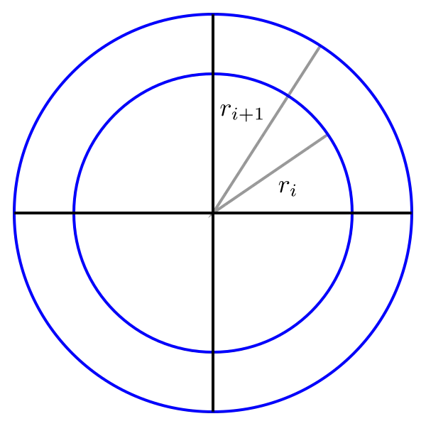
Consider a polar rectangle $R\text{,}$ with $r$ between $r_i$ and $r_{i+1}$ and $\theta$ between $\theta_j$ and $\theta_{j+1}$ as shown at left in Figure $11.5.2$. Let $\Delta r = r_{i+1}-r_i$ and $\Delta \theta = \theta_{j+1}-\theta_j\text{.}$ Let $\Delta A$ be the area of this region.

1. Explain why the area $\Delta A$ in polar coordinates is not $\Delta r \, \Delta \theta\text{.}$
2. Now find $\Delta A$ by the following steps:
   1. Find the area of the annulus (the washer-like region) between $r_i$ and $r_{i+1}\text{,}$ as shown at right in Figure $11.5.2$. This area will be in terms of $r_i$ and $r_{i+1}\text{.}$
   2. Observe that the region $R$ is only a portion of the annulus, so the area $\Delta A$ of $R$ is only a fraction of the area of the annulus. For instance, if $\theta_{i+1} - \theta_i$ were $\frac{\pi}{4}\text{,}$ then the resulting wedge would be
      $$\frac{ \frac{\pi}{4} }{2\pi} = \frac{1}{8}$$

      of the entire annulus. In this more general context, using the wedge between the two noted angles, what fraction of the area of the annulus is the area $\Delta A\text{?}$

   3. Write an expression for $\Delta A$ in terms of $r_i\text{,}$ $r_{i+1}\text{,}$ $\theta_j\text{,}$ and $\theta_{j+1}\text{.}$
   4. Finally, write the area $\Delta A$ in terms of $r_i\text{,}$ $r_{i+1}\text{,}$ $\Delta r\text{,}$ and $\Delta \theta\text{,}$ where each quantity appears only once in the expression. (Hint: Think about how to factor a difference of squares.)
3. As we take the limit as $\Delta r$ and $\Delta \theta$ go to 0, $\Delta r$ becomes $dr\text{,}$ $\Delta \theta$ becomes $d \theta\text{,}$ and $\Delta A$ becomes $dA\text{,}$ the area element. Using your work in (iv), write $dA$ in terms of $r\text{,}$ $dr\text{,}$ and $d \theta\text{.}$

From the result of Activity $11.5.3$, we see when we convert an integral from rectangular coordinates to polar coordinates, we must not only convert $x$ and $y$ to being in terms of $r$ and $\theta\text{,}$ but we also have to change the area element to $dA = r \, dr \, d\theta$ in polar coordinates. As we saw in Activity $11.5.3$, the reason the additional factor of $r$ in the polar area element is due to the fact that in polar coordinates, the cross sectional area element increases as $r$ increases, while the cross sectional area element in rectangular coordinates is constant. So, given a double integral $\iint_D f(x,y) \, dA$ in rectangular coordinates, to write a corresponding iterated integral in polar coordinates, we replace $x$ with $r \cos(\theta)\text{,}$ $y$ with $r \sin(\theta)$ and $dA$ with $r \, dr \, d\theta\text{.}$ Of course, we need to describe the region $D$ in polar coordinates as well. To summarize:

Double integrals in polar coordinates

The double integral $\iint_D f(x,y) \, dA$ in rectangular coordinates can be converted to a double integral in polar coordinates as $\iint_D f(r\cos(\theta), r\sin(\theta)) \, r \, dr \, d\theta\text{.}$

Example $11.5.3$

Let $f(x,y) = e^{x^2+y^2}$ on the disk $D = \{(x,y) : x^2 + y^2 \leq 1\}\text{.}$ We will evaluate $\iint_D f(x,y) \, dA\text{.}$

In rectangular coordinates the double integral $\iint_D f(x,y) \, dA$ can be written as the iterated integral

$$\iint_D f(x,y) \, dA = \int_{x=-1}^{x=1} \int_{y=-\sqrt{1-x^2}}^{y=\sqrt{1-x^2}} e^{x^2+y^2} \, dy \, dx.$$

We cannot evaluate this iterated integral, because $e^{x^2 + y^2}$ does not have an elementary antiderivative with respect to either $x$ or $y\text{.}$ However, since $r^2=x^2+y^2$ and the region $D$ is circular, it is natural to wonder whether converting to polar coordinates will allow us to evaluate the new integral. To do so, we replace $x$ with $r \cos(\theta)\text{,}$ $y$ with $r \sin(\theta)\text{,}$ and $dy \, dx$ with $r \, dr \, d\theta$ to obtain

$$\iint_D f(x,y) \, dA = \iint_D e^{r^2} \, r \, dr \, d\theta.$$

The disc $D$ is described in polar coordinates by the constraints $0 \leq r \leq 1$ and $0 \leq \theta \leq 2\pi\text{.}$ Therefore, it follows that

$$\iint_D e^{r^2} \, r \, dr \, d\theta = \int_{\theta=0}^{\theta = 2\pi} \int_{r=0}^{r=1} e^{r^2} \, r \, dr \, d\theta.$$

We can evaluate the resulting iterated polar integral as follows:

$$\begin{align*} \int_{\theta=0}^{\theta = 2\pi} \int_{r=0}^{r=1} e^{r^2} \, r \, dr \, d\theta & = \int_{\theta=0}^{2\pi} \left( \frac{1}{2}e^{r^2}\biggm|_{r=0}^{r=1} \right) \, d\theta\\[4pt] & = \frac{1}{2} \int_{\theta=0}^{\theta = 2\pi} \left( e-1 \right) \, d\theta\\[4pt] & = \frac{1}{2}(e-1) \int_{\theta=0}^{\theta = 2\pi} \, d\theta\\[4pt] & = \frac{1}{2}(e-1)\left[\theta\right]\biggm|_{\theta=0}^{\theta = 2\pi}\\[4pt] & = \pi(e-1). \end{align*}$$

While there is no firm rule for when polar coordinates can or should be used, they are a natural alternative anytime the domain of integration may be expressed simply in polar form, and/or when the integrand involves expressions such as $\sqrt{x^2 + y^2}.$

Activity $11.5.4$

Let $f(x,y) = x+y$ and $D = \{(x,y) : x^2 + y^2 \leq 4\}\text{.}$

1. Sketch the region $D$ and then write the double integral of $f$ over $D$ as an iterated integral in rectangular coordinates.
2. Write the double integral of $f$ over $D$ as an iterated integral in polar coordinates.
3. Evaluate one of the iterated integrals. Why is the final value you found not surprising?

Activity $11.5.5$

Consider the circle given by $x^2 + (y-1)^2 = 1$ as shown in Figure $11.5.4$.

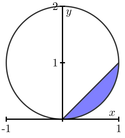
1. Determine a polar curve in the form $r = f(\theta)$ that traces out the circle $x^2 + (y-1)^2 = 1\text{.}$ (Hint: Recall that a circle centered at the origin of radius $r$ can be described by the equations $x = r \cos(\theta)$ and $y = r \sin(\theta)\text{.}$)
2. Find the exact average value of $g(x,y) = \sqrt{x^2 + y^2}$ over the interior of the circle $x^2 + (y-1)^2 = 1\text{.}$
3. Find the volume under the surface $h(x,y) = x$ over the region $D\text{,}$ where $D$ is the region bounded above by the line $y=x$ and below by the circle (this is the shaded region in Figure $11.5.4$).
4. Explain why in both (b) and (c) it is advantageous to use polar coordinates.

Summary

• The polar representation of a point $P$ is the ordered pair $(r,\theta)$ where $r$ is the distance from the origin to $P$ and $\theta$ is the angle the ray through the origin and $P$ makes with the positive $x$-axis.
• The polar coordinates $r$ and $\theta$ of a point $(x,y)$ in rectangular coordinates satisfy
  $$r = \sqrt{x^2+y^2} \ \ \ \ \ \text{ and } \ \ \ \ \ \tan(\theta) = \frac{y}{x};$$

  the rectangular coordinates $x$ and $y$ of a point $(r,\theta)$ in polar coordinates satisfy

  $$x = r\cos(\theta) \ \ \ \ \ \text{ and } \ \ \ \ \ y = r\sin(\theta).$$
• The area element $dA$ in polar coordinates is determined by the area of a slice of an annulus and is given by
  $$dA = r \, dr \, d\theta.$$
• To convert the double integral ${\iint_D f(x,y) \, dA}$ to an iterated integral in polar coordinates, we substitute $r \cos(\theta)$ for $x\text{,}$ $r \sin(\theta)$ for $y\text{,}$ and $r \, dr \, d\theta$ for $dA$ to obtain the iterated integral
  $${\iint_D f(r\cos(\theta), r\sin(\theta)) \, r \, dr \, d\theta}.$$