5Motivating Questions
- What do we mean by the derivative of a vector-valued function and how do we calculate it?
- What does the derivative of a vector-valued function measure?
- What do we mean by the integral of a vector-valued function and how do we compute it?
- How do we describe the motion of a projectile if the only force acting on the object is acceleration due to gravity?
A vector-valued function determines a curve in space as the collection of terminal points of the vectors If the curve is smooth, it is natural to ask whether has a derivative. In the same way, our experiences with integrals in single-variable calculus prompt us to wonder what the integral of a vector-valued function might be and what it might tell us. We explore both of these questions in detail in this section.
For now, let's recall some important ideas from calculus I. Given a function that measures the position of an object moving along an axis, its derivative, is defined by
and measures the instantaneous rate of change of with respect to time. In particular, for a fixed value measures the velocity of the moving object, as well as the slope of the tangent line to the curve at the point
As we work with vector-valued functions, we will strive to update these ideas and perspectives into the context of curves in space and outputs that are vectors.
Preview Activity
Let describe the path traveled by an object at time
- Use appropriate technology to help you sketch the graph of the vector-valued function and then locate and label the point on the graph when
- Recall that for functions of a single variable, the derivative of a sum is the sum of the derivatives; that is, With this idea in mind and viewing and as constant vectors, what do you expect the derivative of to be? Write a proposed formula for
- Use your result from part (b) to compute Sketch this vector as emanating from the point on the graph of when , and explain what you think tells us about the object's motion.
The Derivative
In single variable calculus, we define the derivative, of a given function by
provided the limit exists. At a given value of measures the instantaneous rate of change of and also tells us the slope of the tangent line to the curve at the point The definition of the derivative extends naturally to vector-valued functions and curves in space.
Definition : Derivative of a Vector-valued Function
The derivative of a vector-valued function is defined to be
for those values of at which the limit exists. We also use the notation and for
Activity
Let's investigate how we can interpret the derivative Let be the vector-valued function whose graph is shown in Figure , and let be a scalar that represents a small change in time. The vector is the blue vector in Figure and is the green vector.
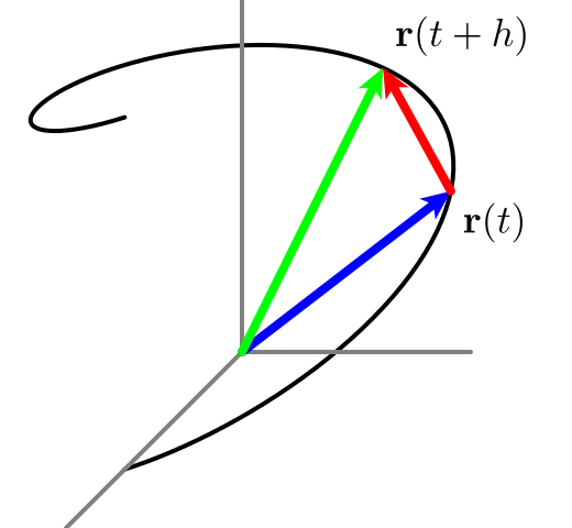
- Is the quantity a vector or a scalar? Identify this object in Figure .
- Is a vector or a scalar? Sketch a representative vector with in Figure .
- Think of as providing the position of an object moving along the curve these vectors trace out. What do you think that the vector measures? Why? (Hint: You might think analogously about difference quotients such as or from calculus I.)
- Figure presents three snapshots of the vectors as we let Write 2-3 sentences to describe key attributes of the vector
(Hint: Compare to limits such as or from calculus I, keeping in mind that in three dimensions there is no general concept of slope.)
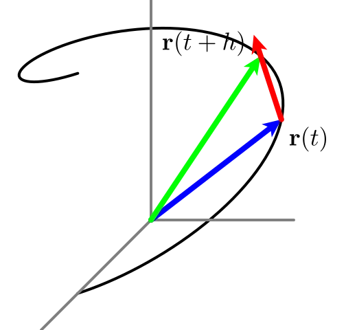
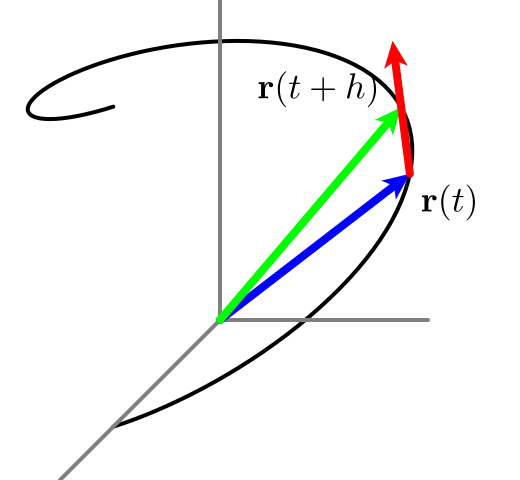
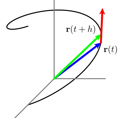
As Activity indicates, if determines the position of an object at time then represents the average rate of change in the position of the object over the interval which is also the average velocity of the object on this interval. Thus, the derivative
is the instantaneous rate of change of at time (for those values of for which the limit exists), so is the instantaneous velocity of the object at time Furthermore, we can interpret the derivative as the direction vector of the line tangent to the graph of at the value
Similarly,
is the instantaneous rate of change of the velocity of the object at time for those values of for which the limits exists, and thus is the acceleration of the moving object.
Note well: Both the velocity and acceleration are vector quantities: they have magnitude and direction. By contrast, the magnitude of the velocity vector, which is the speed of the object at time is a scalar quantity.
Computing Derivatives
As we learned in single variable calculus, computing derivatives from the definition is often difficult. Fortunately, properties of the limit make it straightforward to calculate the derivative of a vector-valued function similar to how we developed shortcut differentiation rules in calculus I. To see why, recall that the limit of a sum is the sum of the limits, and that we can remove constant factors from limits. Thus, as we observed in a particular example in Preview Activity , if it follows that
<span class="katex"><math xmlns="http://www.w3.org/1998/Math/MathML" display="block"><semantics><mtable rowspacing="0.25em" columnalign="right left" columnspacing="0em"><mtr><mtd><mstyle scriptlevel="0" displaystyle="true"><mrow><msup><mi mathvariant="bold">r</mi><mo mathvariant="normal" lspace="0em" rspace="0em">′</mo></msup><mo stretchy="false">(</mo><mi>t</mi><mo stretchy="false">)</mo><mo>=</mo><mpadded width="0px"><mphantom><mo stretchy="false">(</mo></mphantom></mpadded></mrow></mstyle></mtd><mtd><mstyle scriptlevel="0" displaystyle="true"><mrow><mrow></mrow><munder><mrow><mi>lim</mi><mo></mo></mrow><mrow><mi>h</mi><mo>→</mo><mn>0</mn></mrow></munder><mfrac><mrow><mi mathvariant="bold">r</mi><mo stretchy="false">(</mo><mi>t</mi><mo>+</mo><mi>h</mi><mo stretchy="false">)</mo><mo>−</mo><mi mathvariant="bold">r</mi><mo stretchy="false">(</mo><mi>t</mi><mo stretchy="false">)</mo></mrow><mi>h</mi></mfrac></mrow></mstyle></mtd></mtr><mtr><mtd><mstyle scriptlevel="0" displaystyle="true"><mrow><mo>=</mo><mpadded width="0px"><mphantom><mo stretchy="false">(</mo></mphantom></mpadded></mrow></mstyle></mtd><mtd><mstyle scriptlevel="0" displaystyle="true"><mrow><mrow></mrow><munder><mrow><mi>lim</mi><mo></mo></mrow><mrow><mi>h</mi><mo>→</mo><mn>0</mn></mrow></munder><mfrac><mrow><mo stretchy="false">[</mo><mi>x</mi><mo stretchy="false">(</mo><mi>t</mi><mo>+</mo><mi>h</mi><mo stretchy="false">)</mo><mo>−</mo><mi>x</mi><mo stretchy="false">(</mo><mi>t</mi><mo stretchy="false">)</mo><mo stretchy="false">]</mo><mi mathvariant="bold">i</mi><mo>+</mo><mo stretchy="false">[</mo><mi>y</mi><mo stretchy="false">(</mo><mi>t</mi><mo>+</mo><mi>h</mi><mo stretchy="false">)</mo><mo>−</mo><mi>y</mi><mo stretchy="false">(</mo><mi>t</mi><mo stretchy="false">)</mo><mo stretchy="false">]</mo><mi mathvariant="bold">j</mi><mo>+</mo><mo stretchy="false">[</mo><mi>z</mi><mo stretchy="false">(</mo><mi>t</mi><mo>+</mo><mi>h</mi><mo stretchy="false">)</mo><mo>−</mo><mi>z</mi><mo stretchy="false">(</mo><mi>t</mi><mo stretchy="false">)</mo><mo stretchy="false">]</mo><mi mathvariant="bold">k</mi></mrow><mi>h</mi></mfrac></mrow></mstyle></mtd></mtr><mtr><mtd><mstyle scriptlevel="0" displaystyle="true"><mrow><mo>=</mo><mpadded width="0px"><mphantom><mo stretchy="false">(</mo></mphantom></mpadded></mrow></mstyle></mtd><mtd><mstyle scriptlevel="0" displaystyle="true"><mrow><mrow></mrow><mrow><mo fence="true">(</mo><munder><mrow><mi>lim</mi><mo></mo></mrow><mrow><mi>h</mi><mo>→</mo><mn>0</mn></mrow></munder><mfrac><mrow><mi>x</mi><mo stretchy="false">(</mo><mi>t</mi><mo>+</mo><mi>h</mi><mo stretchy="false">)</mo><mo>−</mo><mi>x</mi><mo stretchy="false">(</mo><mi>t</mi><mo stretchy="false">)</mo></mrow><mi>h</mi></mfrac><mo fence="true">)</mo></mrow><mi mathvariant="bold">i</mi><mo>+</mo><mrow><mo fence="true">(</mo><munder><mrow><mi>lim</mi><mo></mo></mrow><mrow><mi>h</mi><mo>→</mo><mn>0</mn></mrow></munder><mfrac><mrow><mi>y</mi><mo stretchy="false">(</mo><mi>t</mi><mo>+</mo><mi>h</mi><mo stretchy="false">)</mo><mo>−</mo><mi>y</mi><mo stretchy="false">(</mo><mi>t</mi><mo stretchy="false">)</mo></mrow><mi>h</mi></mfrac><mo fence="true">)</mo></mrow><mi mathvariant="bold">j</mi></mrow></mstyle></mtd></mtr><mtr><mtd><mstyle scriptlevel="0" displaystyle="true"><mpadded width="0px"><mphantom><mo stretchy="false">(</mo></mphantom></mpadded></mstyle></mtd><mtd><mstyle scriptlevel="0" displaystyle="true"><mrow><mrow></mrow><mo>+</mo><mrow><mo fence="true">(</mo><munder><mrow><mi>lim</mi><mo></mo></mrow><mrow><mi>h</mi><mo>→</mo><mn>0</mn></mrow></munder><mfrac><mrow><mi>z</mi><mo stretchy="false">(</mo><mi>t</mi><mo>+</mo><mi>h</mi><mo stretchy="false">)</mo><mo>−</mo><mi>z</mi><mo stretchy="false">(</mo><mi>t</mi><mo stretchy="false">)</mo></mrow><mi>h</mi></mfrac><mo fence="true">)</mo></mrow><mi mathvariant="bold">k</mi></mrow></mstyle></mtd></mtr><mtr><mtd><mstyle scriptlevel="0" displaystyle="true"><mpadded width="0px"><mphantom><mo stretchy="false">(</mo></mphantom></mpadded></mstyle></mtd><mtd><mstyle scriptlevel="0" displaystyle="true"><mrow><mrow></mrow><mo>=</mo><msup><mi>x</mi><mo mathvariant="normal" lspace="0em" rspace="0em">′</mo></msup><mo stretchy="false">(</mo><mi>t</mi><mo stretchy="false">)</mo><mi mathvariant="bold">i</mi><mo>+</mo><msup><mi>y</mi><mo mathvariant="normal" lspace="0em" rspace="0em">′</mo></msup><mo stretchy="false">(</mo><mi>t</mi><mo stretchy="false">)</mo><mi mathvariant="bold">j</mi><mo>+</mo><msup><mi>z</mi><mo mathvariant="normal" lspace="0em" rspace="0em">′</mo></msup><mo stretchy="false">(</mo><mi>t</mi><mo stretchy="false">)</mo><mi mathvariant="bold">k</mi><mi mathvariant="normal">.</mi></mrow></mstyle></mtd></mtr></mtable><annotation encoding="application/x-tex">\begin{align*} \mathbf{r}'(t) = \mathstrut & \lim_{h \to 0} \frac{\mathbf{r}(t+h)-\mathbf{r}(t)}{h}\\[4pt] = \mathstrut & \lim_{h \to 0} \frac{[x(t+h)-x(t)] \mathbf{i} + [y(t+h)-y(t)] \mathbf{j} + [z(t+h)-z(t)] \mathbf{k}}{h}\\[4pt] = \mathstrut & \left(\lim_{h \to 0} \frac{x(t+h)-x(t)}{h} \right) \mathbf{i} + \left( \lim_{h \to 0} \frac{y(t+h)-y(t)}{h} \right) \mathbf{j}\\[4pt] \mathstrut & + \left( \lim_{h \to 0} \frac{z(t+h)-z(t)}{h} \right)\mathbf{k}\\[4pt] \mathstrut & = x'(t)\mathbf{i} + y'(t) \mathbf{j} + z'(t) \mathbf{k}. \end{align*}</annotation></semantics></math></span>
Thus, we can calculate the derivative of a vector-valued function by simply differentiating its components.
The derivative of a vector-valued function
If then
for those values of at which and are differentiable.
Activity
For each of the following vector-valued functions, find
In first-semester calculus, we developed several important differentiation rules, including the constant multiple, product, quotient, and chain rules. For instance, recall that we formally state the product rule as
There are several analogous rules for vector-valued functions, including a product rule for scalar functions and vector-valued functions. These rules, which are easily verified, are summarized as follows.
Properties of derivatives of vector-valued functions
Let be a differentiable real-valued function of a real variable and let and be differentiable vector-valued functions of the real variable Then
Note well. When applying these properties, use care to interpret the quantities involved as either scalars or vectors. For example, defines a scalar function because we have taken the dot product of two vector-valued functions. However, defines a vector-valued function since we have taken the cross product of two vector-valued functions.
Activity
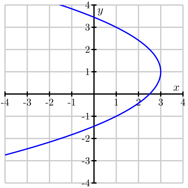
The left side of Figure shows the curve described by the vector-valued function defined by
- Find the object's velocity
- Find the object's acceleration
- Indicate on the left of Figure the object's position, velocity and acceleration at the times Draw the velocity and acceleration vectors with their tails placed at the object's position.
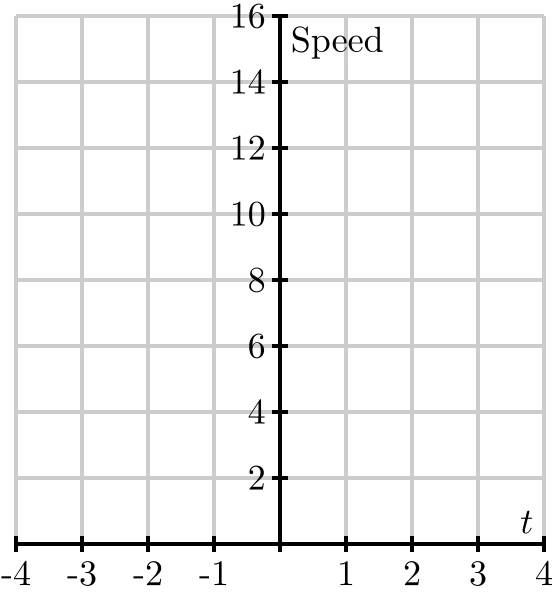
- Recall that the speed is Find the object's speed and graph it as a function of time on the right of Figure . When is the object's speed the slowest? When is the speed increasing? When is it decreasing?
- What seems to be true about the angle between and when the speed is at a minimum? What is the angle between and when the speed is increasing? when the speed is decreasing?
- Since the square root is an increasing function, we see that the speed increases precisely when is increasing. Use the product rule for the dot product to express in terms of the velocity and acceleration Use this to explain why the speed is increasing when and decreasing when Compare this to part (d).
- Show that the speed's rate of change is
Tangent Lines
One of the most important ideas in first-semester calculus is that a differentiable function is locally linear: that is, when viewed up close, the curve generated by a differentiable function looks very much like a line. Indeed, when we zoom in sufficiently far on a particular point, the curve looks indistinguishable from its tangent line.
In the same way, we expect that a smooth curve in 3-space will be locally linear. In the following activity, we investigate how to find the tangent line to such a curve. Recall from our work in Section 9.5 that the vector equation of a line that passes through the point at the tip of the vector in the direction of the vector can be written as
In parametric form, the line is given by
Activity
Let
Sketch the curve using some appropriate tool.
- Determine the coordinates of the point on the curve traced out by when
- Find a direction vector for the line tangent to the graph of at the point where
- Find the parametric equations of the line tangent to the graph of when
- Sketch a plot of the curve and its tangent line near the point where In addition, include a sketch of What is the important role of in this activity?
We see that our work in Activity can be generalized. Given a differentiable vector-valued function the tangent line to the curve at the input value is given by
Here we see that because the tangent line is determined entirely by a given point and direction, the point is provided by the function evaluated at while the direction is provided by the derivative, again evaluated at Note how analogous the formula for is to the tangent line approximation from single-variable calculus: in that context, for a given function at a value we found that the tangent line can be expressed by the linear function whose formula is
Equation () for the tangent line to the vector-valued function is nearly identical. Indeed, because there are multiple parameterizations for a single line, it is even possible to write the parameterization as
(For example, in Equation (), so the line's parameterization “starts” at When we write the parameterization in the form of Equation (), so the line's parameterization “starts” at )
As we will learn more in Chapter 10, a smooth surface in 3-space is also locally linear. That means that the surface will look like a plane, which we call its tangent plane, as we zoom in on the graph. It is possible to use tangent lines to traces of the surface to generate a formula for the tangent plane; see Exercise .15 at the end of this section for more details.
Integrating a Vector-Valued Function
Recall from single variable calculus that an antiderivative of a function of the independent variable is a function that satisfies We then defined the indefinite integral to be the general antiderivative of Recall that the general antiderivative includes an added constant in order to indicate that the general antiderivative is in fact an entire family of functions. We can do the similar work with vector-valued functions.
Definition
An antiderivative of a vector-valued function is a vector-valued function such that
The indefinite integral of a vector-valued function is the general antiderivative of and represents the collection of all antiderivatives of
The same reasoning that allows us to differentiate a vector-valued function componentwise applies to integrating as well. Recall that the integral of a sum is the sum of the integrals and also that we can remove constant factors from integrals. So, given it follows that we can integrate componentwise. Expressed more formally,
Integrating a vector-valued function
If then
In light of being able to integrate and differentiate componentwise with vector-valued functions, we can solve many problems that are analogous to those we encountered in single-variable calculus. For instance, recall problems where we were given an object moving along an axis with velocity function and an initial position In that context, we were able to differentiate in order to find acceleration, and integrate and use the initial condition in order to find the position function In the following activity, we explore similar ideas with vector-valued functions.
Activity
Suppose a moving object in space has its velocity given by
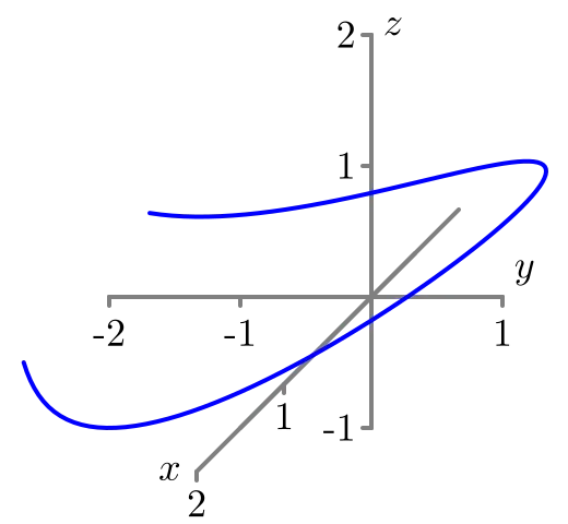
A graph of the position of the object for times in is shown in Figure . Suppose further that the object is at the point at time
- Determine the acceleration of the object at time
- Determine position of the object at time
- Compute and sketch the position, velocity, and acceleration vectors of the object at time using Figure .
- Finally, determine the vector equation for the tangent line, that is tangent to the position curve at
Projectile Motion
Any time that an object is launched into the air with a given velocity and launch angle, the path the object travels is determined almost exclusively by the force of gravity. Whether in sports such as archery or shotput, in military applications with artillery, or in important fields like firefighting, it is important to be able to know when and where a launched projectile will land. We can use our knowledge of vector-valued functions in order to completely determine the path traveled by an object that is launched from a given position at a given angle from the horizontal with a given initial velocity.
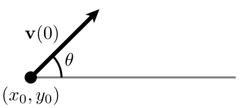
Assume we fire a projectile from a launcher and the only force acting on the fired object is the force of gravity pulling down on the object. That is, we assume no effect due to spin, wind, or air resistance. With these assumptions, the motion of the object will be planar, so we can also assume that the motion occurs in two-dimensional space. Suppose we launch the object from an initial position at an angle with the positive -axis as illustrated in Figure , and that we fire the object with an initial speed of where is the velocity vector of the object at time Assume is the positive constant acceleration force due to gravity, which acts to pull the fired object toward the ground (in the negative direction). Note particularly that there is no external force acting on the object to move it in the direction.
We first observe that since gravity only acts in the downward direction and that the acceleration due to gravity is constant, the acceleration vector is That is, We may use this fact about acceleration, together with the initial position and initial velocity in order to fully determine the position of the object at time In Exercise , you can work through the details to show that the following general formula holds.
The motion of a projectile
If an object is launched from a point with initial velocity at an angle with the horizontal, then the position of the object at time is given by
This assumes that the only force acting on the object is the acceleration due to gravity.
Summary
- If is a vector-valued function, then the derivative of is defined by
for those values of at which the limit exists, and is computed componentwise by the formula
for those values of at which and are differentiable, where
- The derivative of the vector-valued function tells us the instantaneous rate of change of with respect to time, which can be interpreted as a direction vector for the line tangent to the graph of at the point or also as the instantaneous velocity of an object traveling along the graph defined by at time
- An antiderivative of is a vector-valued function such that The indefinite integral of a vector-valued function is the general antiderivative of (which is a collection of all of the antiderivatives of with any two antiderivatives differing by at most a constant vector). Moreover, if then
- If an object is launched from a point with initial velocity at an angle with the horizontal, then the position of the object at time is given by
provided that that the only force acting on the object is the acceleration due to gravity.