Active Calculus · 9: Multivariable and Vector Functions

9.3: Dot Product

Motivating Questions
  • How is the dot product of two vectors defined and what geometric information does it tell us?
  • How can we tell if two vectors in Rn\mathbb{R}^n are perpendicular?
  • How do we find the projection of one vector onto another?

In the last section, we considered vector addition and scalar multiplication and found that each operation had a natural geometric interpretation. In this section, we will introduce a means of multiplying vectors.

Preview Activity 9.3.19.3.1

For two-dimensional vectors u=⟨u1,u2⟩\mathbf{u} =\langle u_1,u_2\rangle and v=⟨v1,v2⟩,\mathbf{v}=\langle v_1, v_2\rangle\text{,} the dot product is simply the scalar obtained by

u⋅v=u1v1+u2v2. \mathbf{u} \cdot \mathbf{v} = u_1v_1 + u_2v_2.

a. If u=⟨3,4⟩\mathbf{u} =\langle 3, 4\rangle and v=⟨−2,1⟩,\mathbf{v}=\langle -2, 1\rangle\text{,} find the dot product u⋅v.\mathbf{u} \cdot \mathbf{v}\text{.}

b. Find i⋅j\mathbf{i} \cdot \mathbf{j} and i⋅j.\mathbf{i} \cdot \mathbf{j}\text{.}

c. If u=⟨3,4⟩,\mathbf{u}=\langle 3, 4\rangle\text{,} find u⋅u.\mathbf{u} \cdot \mathbf{u} \text{.} How is this related to ∣u∣?|\mathbf{u}|\text{?}

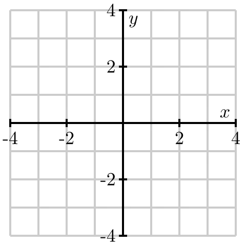
d. On the axes in Figure 9.3.19.3.1, plot the vectors u=⟨1,3⟩\mathbf{u}=\langle 1, 3\rangle and v=⟨−3,1⟩.\mathbf{v}=\langle -3, 1\rangle\text{.} Then, find u⋅v.\mathbf{u} \cdot \mathbf{v}\text{.} What is the angle between these vectors?

fig_9_3_preview_1.svg

Figure 9.3.19.3.1. For part (d)

e. On the axes in Figure 9.3.29.3.2, plot the vector u=⟨1,3⟩.\mathbf{u} =\langle 1, 3\rangle\text{.}

fig_9_3_preview_1.svg

Figure 9.3.29.3.2. For part (e)

For each of the following vectors v,\mathbf{v}\text{,} plot the vector on Figure 9.3.29.3.2 and then compute the dot product u⋅v.\mathbf{u} \cdot \mathbf{v}\text{.}

  • v=⟨3,2⟩.\mathbf{v}=\langle 3, 2 \rangle\text{.}
  • v=⟨3,0⟩.\mathbf{v}=\langle 3, 0 \rangle\text{.}
  • v=⟨3,−1⟩.\mathbf{v}=\langle 3,-1 \rangle\text{.}
  • v=⟨3,−2⟩.\mathbf{v}=\langle 3,-2 \rangle\text{.}
  • v=⟨3,−4⟩.\mathbf{v}=\langle 3,-4 \rangle\text{.}

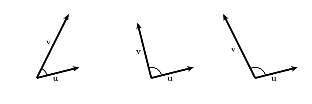
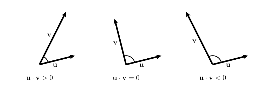
f. Based upon the previous part of this activity, what do you think is the sign of the dot product in the following three cases shown in Figure 9.3.39.3.3?

fig_9_3_preview_2.svg

Figure 9.3.39.3.3. For part (f)

The Dot Product

The definition of the dot product for vectors in R2\mathbb{R}^2 given in Preview Activity 9.3.19.3.1 can be extended to vectors in Rn.\mathbb{R}^n\text{.}

Definition 9.3.49.3.4

The dot product of vectors u=⟨u1,u2,…,un⟩\mathbf{u}=\langle u_1, u_2,\ldots,u_n\rangle and v=⟨v1,v2,…,vn⟩\mathbf{v}=\langle v_1, v_2,\ldots,v_n\rangle in Rn\mathbb{R}^n is the scalar

u⋅v=u1v1+u2v2+…+unvn. \mathbf{u} \cdot \mathbf{v} = u_1v_1+u_2v_2 + \ldots + u_nv_n.

(As we will see shortly, the dot product arises in physics to calculate the work done by a vector force in a given direction. It might be more natural to define the dot product in this context, but it is more convenient from a mathematical perspective to define the dot product algebraically and then view work as an application of this definition.)

For instance, we find that

⟨3,0,1⟩⋅⟨−2,1,4⟩=3⋅(−2)+0⋅1+1⋅4=−6+0+4=−2. \langle 3, 0, 1 \rangle\cdot\langle -2, 1, 4\rangle = 3\cdot(-2) + 0\cdot1 + 1\cdot4 = -6 + 0 + 4 = -2.

Notice that the resulting quantity is a scalar. Our work in Preview Activity 9.3.19.3.1 examined dot products of two-dimensional vectors.

Activity 9.3.29.3.2

Determine each of the following.

  1. ⟨1,2,−3⟩⋅⟨4,−2,0⟩.\langle 1, 2, -3 \rangle \cdot \langle 4, -2, 0 \rangle\text{.}
  2. ⟨0,3,−2,1⟩⋅⟨5,−6,0,4⟩\displaystyle \langle 0, 3, -2, 1 \rangle \cdot \langle 5, -6, 0, 4 \rangle

The dot product is a natural way to define a product of two vectors. In addition, it behaves in ways that are similar to the product of, say, real numbers.

Properties of the dot product

Let u,\mathbf{u}\text{,} v,\mathbf{v}\text{,} and w\mathbf{w} be vectors in Rn.\mathbb{R}^n\text{.} Then

  1. u⋅v=v⋅u\mathbf{u} \cdot \mathbf{v} = \mathbf{v} \cdot \mathbf{u} (the dot product is commutative), and
  2. (u+v)⋅w=(u⋅w)+(v⋅w).(\mathbf{u} + \mathbf{v}) \cdot \mathbf{w} = (\mathbf{u} \cdot \mathbf{w}) + (\mathbf{v} \cdot \mathbf{w})\text{.}
  3. if cc is a scalar, then (cu)⋅w=c(u⋅w).(c\mathbf{u}) \cdot \mathbf{w} = c(\mathbf{u} \cdot \mathbf{w})\text{.}

Moreover, the dot product gives us valuable geometric information about the vectors and their relative orientation. For instance, let's consider what happens when we dot a vector with itself:

u⋅u=⟨u1,u2,…,un⟩⋅⟨u1,u2,…,un⟩=u12+u22+…+un2=∣u∣2. \mathbf{u} \cdot \mathbf{u} = \langle u_1,u_2,\ldots,u_n \rangle \cdot \langle u_1,u_2,\ldots,u_n \rangle = u_1^2 + u_2^2 + \ldots + u_n^2 = |\mathbf{u}|^2.

In other words, the dot product of a vector with itself gives the square of the length of the vector: u⋅u=∣u∣2.\mathbf{u} \cdot \mathbf{u}=|\mathbf{u}|^2\text{.}

The angle between vectors

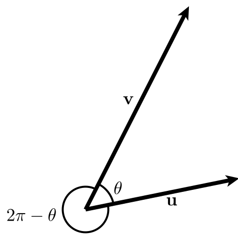
The dot product can help us understand the angle between two vectors. For instance, if we are given two vectors u\mathbf{u} and v,\mathbf{v}\text{,} there are two angles that these vectors create, as depicted at left in Figure 9.3.49.3.4. We will call θ,\theta\text{,} the smaller of these angles, the angle between these vectors. Notice that θ\theta lies between 0 and π.\pi\text{.}

fig_9_3_angle_1.svg fig_9_3_angle_2.svg

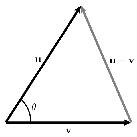
Figure 9.3.49.3.4. Left: The angle between u\mathbf{u} and v.\mathbf{v}\text{.} Right: The triangle formed by u,\mathbf{u} \text{,} v,\mathbf{v} \text{,} and u−v.\mathbf{u} - \mathbf{v} \text{.}

To determine this angle, we may apply the Law of Cosines to the triangle shown at right in Figure 9.3.49.3.4.

Using the fact that the dot product of a vector with itself gives us the square of its length, together with the properties of the dot product, we find:

∣u−v∣2=(∣u∣2+∣v∣2−2∣u∣∣v∣cos⁡(θ)(u−v)⋅(u−v)=(u⋅u+v⋅v−2∣u∣∣v∣cos⁡(θ)u⋅(u−v)−v⋅(u−v)=(u⋅u+v⋅v−2∣u∣∣v∣cos⁡(θ)u⋅u−2u⋅v+v⋅v=(u⋅u+v⋅v−2∣u∣∣v∣cos⁡(θ)−2u⋅v=(−2∣u∣∣v∣cos⁡(θ)u⋅v=(∣u∣∣v∣cos⁡(θ).\begin{align*} |\mathbf{u}-\mathbf{v}|^2 =\mathstrut & |\mathbf{u}|^2 + |\mathbf{v}|^2 - 2|\mathbf{u}||\mathbf{v}|\cos(\theta)\\[4pt] (\mathbf{u}-\mathbf{v})\cdot(\mathbf{u}-\mathbf{v}) =\mathstrut & \mathbf{u} \cdot \mathbf{u} + \mathbf{v} \cdot \mathbf{v} - 2|\mathbf{u}||\mathbf{v}|\cos(\theta)\\[4pt] \mathbf{u} \cdot (\mathbf{u}-\mathbf{v}) - \mathbf{v}\cdot(\mathbf{u}-\mathbf{v})=\mathstrut & \mathbf{u}\cdot\mathbf{u} + \mathbf{v} \cdot \mathbf{v} - 2|\mathbf{u}| |\mathbf{v}|\cos(\theta)\\[4pt] \mathbf{u} \cdot \mathbf{u} - 2\mathbf{u} \cdot \mathbf{v} + \mathbf{v} \cdot \mathbf{v} =\mathstrut & \mathbf{u} \cdot \mathbf{u} + \mathbf{v} \cdot \mathbf{v} - 2|\mathbf{u}||\mathbf{v}|\cos(\theta)\\[4pt] -2\mathbf{u} \cdot \mathbf{v} =\mathstrut & -2|\mathbf{u}||\mathbf{v}|\cos(\theta)\\[4pt] \mathbf{u} \cdot \mathbf{v} =\mathstrut & |\mathbf{u}||\mathbf{v}|\cos(\theta). \end{align*}

To summarize, we have the important relationship

u⋅v=u1v1+u2v2+…+unvn=∣u∣∣v∣cos⁡(θ).(9.3.1) \mathbf{u} \cdot \mathbf{v} = u_1v_1+u_2v_2 + \ldots + u_nv_n = |\mathbf{u}||\mathbf{v}|\cos(\theta).\tag{9.3.19.3.1}

It is sometimes useful to think of Equation (9.3.19.3.1) as giving us an expression for the angle between two vectors:

θ=cos⁡−1(u⋅v∣u∣∣v∣). \theta = \cos^{-1}\left(\frac{\mathbf{u} \cdot \mathbf{v}}{|\mathbf{u}||\mathbf{v}|}\right).

The real beauty of this expression is this: the dot product is a very simple algebraic operation to perform yet it provides us with important geometric information — namely the angle between the vectors — that would be difficult to determine otherwise.

Activity 9.3.39.3.3

Determine each of the following.

  1. The length of the vector u=⟨1,2,−3⟩\mathbf{u}=\langle 1,2,-3\rangle using the dot product.
  2. The angle between the vectors u=⟨1,2⟩\mathbf{u} =\langle 1, 2 \rangle and v=⟨4,−1⟩\mathbf{v} = \langle 4, -1 \rangle to the nearest tenth of a degree.
  3. The angle between the vectors y=⟨1,2,−3⟩\mathbf{y} =\langle 1, 2, -3 \rangle and z=⟨−2,1,1⟩\mathbf{z} = \langle -2, 1, 1 \rangle to the nearest tenth of a degree.
  4. If the angle between the vectors u\mathbf{u} and v\mathbf{v} is a right angle, what does the expression u⋅v=∣u∣∣v∣cos⁡(θ)\mathbf{u} \cdot \mathbf{v}=|\mathbf{u}||\mathbf{v}|\cos(\theta) say about their dot product?
  5. If the angle between the vectors u\mathbf{u} and v\mathbf{v} is acute—that is, less than π/2\pi/2—what does the expression u⋅v=∣u∣∣v∣cos⁡(θ)\mathbf{u}\cdot \mathbf{v} =|\mathbf{u}||\mathbf{v}|\cos(\theta) say about their dot product?
  6. If the angle between the vectors u\mathbf{u} and v\mathbf{v} is obtuse—that is, greater than π/2\pi/2—what does the expression u⋅v=∣u∣∣v∣cos⁡(θ)\mathbf{u} \cdot \mathbf{v}=|\mathbf{u}||\mathbf{v}|\cos(\theta) say about their dot product?

The Dot Product and Orthogonality

When the angle between two vectors is a right angle, it is frequently the case that something important is happening. In this case, we say the vectors are orthogonal. For instance, orthogonality often plays a role in optimization problems; to determine the shortest path from a point in R3\mathbb{R}^3 to a given plane, we move along a line orthogonal to the plane.

As Activity 9.3.39.3.3 indicates, the dot product provides a simple means to determine whether two vectors are orthogonal to one another. In this case, u⋅v=∣u∣∣v∣cos⁡(π/2)=0,\mathbf{u} \cdot \mathbf{v} =|\mathbf{u}||\mathbf{v}|\cos(\pi/2) = 0\text{,} so we make the following important observation.

The dot product and orthogonality

Two vectors u\mathbf{u} and v\mathbf{v} in Rn\mathbb{R}^n are orthogonal to each other if u⋅v=0.\mathbf{u} \cdot \mathbf{v} = 0\text{.}

More generally, the sign of the dot product gives us useful information about the relative orientation of the vectors. If we remember that

cos⁡(θ)>0(    if θ is an acute angle,cos⁡(θ)=0(    if θ is a right angle, andcos⁡(θ)<0(    if θ is an obtuse angle,\begin{align*} \cos(\theta) \gt 0 \mathstrut & \ \ \ \text{ if } \theta \text{ is an acute angle,}\\[4pt] \cos(\theta) = 0 \mathstrut & \ \ \ \text{ if } \theta \text{ is a right angle, and}\\[4pt] \cos(\theta) \lt 0 \mathstrut & \ \ \ \text{ if } \theta \text{ is an obtuse angle,} \end{align*}

we see that for nonzero vectors u\mathbf{u} and v,\mathbf{v} \text{,}

u⋅v>0(    if θ is an acute angle,u⋅v=0(    if θ is a right angle, andu⋅v<0(    if θ is an obtuse angle.\begin{align*} \mathbf{u} \cdot \mathbf{v} \gt 0 \mathstrut & \ \ \ \text{ if } \theta \text{ is an acute angle,}\\[4pt] \mathbf{u} \cdot \mathbf{v} = 0 \mathstrut & \ \ \ \text{ if } \theta \text{ is a right angle, and}\\[4pt] \mathbf{u} \cdot \mathbf{v} \lt 0 \mathstrut & \ \ \ \text{ if } \theta \text{ is an obtuse angle.} \end{align*}

This is illustrated in Figure 9.3.59.3.5.

fig_9_3_orientations.svg

Figure 9.3.59.3.5. The orientation of vectors

Work, Force, and Displacement

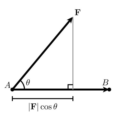
In physics, work is a measure of the energy required to apply a force to an object through a displacement. For instance, Figure 9.3.69.3.6 shows a force F\mathbf{F} displacing an object from point AA to point B.B\text{.} The displacement is then represented by the vector AB→.\overrightarrow{AB}\text{.}

fig_9_3_work_1.svg

Figure 9.3.69.3.6. A force F\mathbf{F} displacing an object.

It turns out that the work required to displace the object is

W=F⋅AB→=∣F∣∣AB→∣cos⁡(θ). W = \mathbf{F}\cdot\overrightarrow{AB} = |\mathbf{F}||\overrightarrow{AB}|\cos(\theta).

This means that the work is determined only by the magnitude of the force applied parallel to the displacement. Consequently, if we are given two vectors u\mathbf{u} and v,\mathbf{v}\text{,} we would like to write u\mathbf{u} as a sum of two vectors, one of which is parallel to v\mathbf{v} and one of which is orthogonal to v.\mathbf{v} \text{.} We take up this task after the next activity.

Activity 9.3.49.3.4

Determine the work done by a 25 pound force acting at a 30∘30^{\circ} angle to the direction of the object's motion, if the object is pulled 10 feet. In addition, is more work or less work done if the angle to the direction of the object's motion is 60∘?60^\circ\text{?}

Projections

fig_9_3_projection_1.svgfig_9_3_projection_2.svg 

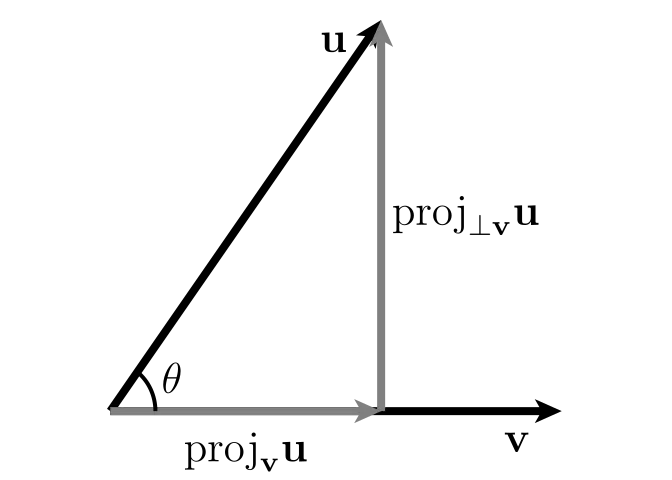
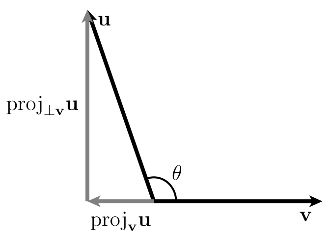
Figure 9.3.79.3.7. Left: projvu.proj_{\mathbf{v}} \mathbf{u} \text{.} Right: projvuproj_{\mathbf{v}} \mathbf{u} when θ>π2.\theta > \frac\pi2\text{.}

Suppose we are given two vectors u\mathbf{u} and v\mathbf{v} as shown at left in Figure 9.3.79.3.7. Motivated by our discussion of work, we would like to write u\mathbf{u} as a sum of two vectors, one of which is parallel to v\mathbf{v} and one of which is orthogonal. That is, we would like to write

u=projvu+proj⊥vu,(9.3.2) \mathbf{u} = proj_{\mathbf{v}}\mathbf{u} + proj_{\perp \mathbf{v}}\mathbf{u},\tag{9.3.29.3.2}

where projvuproj_{\mathbf{v}}\mathbf{u} is parallel to v\mathbf{v} and proj⊥vuproj_{\perp \mathbf{v}}\mathbf{u} is orthogonal to v.\mathbf{v} \text{.} We call the vector projvuproj_{\mathbf{v}}\mathbf{u} the projection of u\mathbf{u} onto v\mathbf{v}. Note that, as the diagram at right in Figure 9.3.89.3.8 illustrates, it is also possible to create a projection even if the angle between the vectors u\mathbf{u} and v\mathbf{v} exceeds π2.\frac\pi2\text{.}

To find the vector projvu,proj_{\mathbf{v}} \mathbf{u}\text{,} we will dot both sides of Equation (9.3.29.3.2) with the vector v,\mathbf{v}\text{,} to find that

u⋅v=((projvu+proj⊥vu)⋅v=((projvu)⋅v+(proj⊥vu)⋅v=((projvu)⋅v.\begin{align*} \mathbf{u} \cdot \mathbf{v} =\mathstrut & (proj_{\mathbf{v}}\mathbf{u} + proj_{\perp \mathbf{v}}\mathbf{u})\cdot \mathbf{v}\\[4pt] =\mathstrut & (proj_{\mathbf{v}}\mathbf{u})\cdot \mathbf{v} + (proj_{\perp \mathbf{v}} \mathbf{u})\cdot \mathbf{v}\\[4pt] =\mathstrut & (proj_{\mathbf{v}}\mathbf{u})\cdot\mathbf{v}. \end{align*}

Notice that (proj⊥vu)⋅v=0(proj_{\perp\mathbf{v}}\mathbf{u})\cdot \mathbf{v} = 0 since proj⊥vuproj_{\perp\mathbf{v}}\mathbf{u} is orthogonal to v.\mathbf{v}\text{.} Also, projvuproj_{\mathbf{v}}\mathbf{u} must be a scalar multiple of v\mathbf{v} since it is parallel to v,\mathbf{v}\text{,} so we will write projvu=sv.proj_{\mathbf{v}}\mathbf{u} = s \mathbf{v} \text{.} It follows that

u⋅v=(projvu)⋅v=sv⋅v, \mathbf{u} \cdot \mathbf{v} =(proj_{\mathbf{v}}\mathbf{u})\cdot \mathbf{v} = s \mathbf{v} \cdot \mathbf{v},

which means that

s=u⋅vv⋅v s = \frac{\mathbf{u} \cdot \mathbf{v}}{\mathbf{v} \cdot \mathbf{v}}

and hence

projvu=u⋅vv⋅vv=u⋅v∣v∣2v proj_{\mathbf{v}}\mathbf{u} = \frac{\mathbf{u} \cdot \mathbf{v}}{\mathbf{v} \cdot \mathbf{v}}\mathbf{v} = \frac{\mathbf{u} \cdot \mathbf{v}}{|\mathbf{v}|^2}\mathbf{v}

It is sometimes useful to write projvuproj_{\mathbf{v}}\mathbf{u} as a scalar times a unit vector in the direction of v.\mathbf{v}\text{.} We call this scalar the component of u\mathbf{u} along v\mathbf{v} and denote it as compvu.comp_{\mathbf{v}}\mathbf{u} \text{.} We therefore have

projvu=u⋅v∣v∣2v=u⋅v∣v∣v∣v∣=compvuv∣v∣, proj_{\mathbf{v}}\mathbf{u} = \frac{\mathbf{u} \cdot \mathbf{v}}{|\mathbf{v}|^2} \mathbf{v} = \frac{\mathbf{u} \cdot \mathbf{v}}{|\mathbf{v}|} \frac{\mathbf{v}}{|\mathbf{v}|}= comp_{\mathbf{v}}\mathbf{u} \frac{\mathbf{v}}{|\mathbf{v}|},

so that

compvu=u⋅v∣v∣. comp_{\mathbf{v}}\mathbf{u} = \frac{\mathbf{u} \cdot \mathbf{v}}{|\mathbf{v}|}.
The dot product and projections

Let u\mathbf{u} and v\mathbf{v} be vectors in Rn.\mathbb{R}^n\text{.} The component of u\mathbf{u} in the direction of v\mathbf{v} is the scalar

compvu=u⋅v∣v∣, comp_{\mathbf{v}} \mathbf{u} = \frac{\mathbf{u} \cdot \mathbf{v}}{|\mathbf{v}|},

and the projection of u\mathbf{u} onto v\mathbf{v} is the vector

projvu=u⋅vv⋅vv. proj_{\mathbf{v}} \mathbf{u} = \frac{\mathbf{u} \cdot \mathbf{v}}{\mathbf{v}\cdot\mathbf{v}} \mathbf{v}.

Moreover, since

u=projvu+proj⊥vu, \mathbf{u} = proj_{\mathbf{v}} \mathbf{u} + proj_{\perp \mathbf{v}} \mathbf{u},

it follows that

proj⊥vu=u−projvu. proj_{\perp \mathbf{v}} \mathbf{u} = \mathbf{u} - proj_{\mathbf{v}} \mathbf{u}.

This shows that once we have computed projvu,proj_{\mathbf{v}} \mathbf{u} \text{,} we can find proj⊥vuproj_{\perp \mathbf{v}} \mathbf{u} simply by calculating the difference of two known vectors.

Activity 9.3.59.3.5

Let u=⟨2,6⟩.\mathbf{u} = \langle 2, 6 \rangle\text{.}

  1. Let v=⟨4,−8⟩.\mathbf{v} = \langle 4, -8 \rangle\text{.} Find compvu,comp_{\mathbf{v}} \mathbf{u} \text{,} projvuproj_{\mathbf{v}} \mathbf{u} and proj⊥vu,proj_{\perp \mathbf{v}} \mathbf{u} \text{,} and draw a picture to illustrate. Finally, express u\mathbf{u} as the sum of two vectors where one is parallel to v\mathbf{v} and the other is perpendicular to v.\mathbf{v}\text{.}
  2. Now let v=⟨−2,4⟩.\mathbf{v} = \langle -2,4 \rangle \text{.} Without doing any calculations, find projvu.proj_{\mathbf{v}} \mathbf{u} \text{.} Explain your reasoning. (Hint: Refer to the picture you drew in part (a).)
  3. Find a vector w\mathbf{w} not parallel to z=⟨3,4⟩\mathbf{z} = \langle 3,4 \rangle such that projzwproj_{\mathbf{z}} \mathbf{w} has length 10.10\text{.} Note that there are infinitely many different answers.

Summary

  • The dot product of two vectors in Rn,\mathbb{R}^n\text{,} u=⟨u1,u2,…,un⟩\mathbf{u} = \langle u_1, u_2, \ldots, u_n \rangle and v=⟨v1,v2,…,vn⟩,\mathbf{v} = \langle v_1, v_2, \ldots, v_n \rangle\text{,} is the scalar
    u⋅v=u1v1+u2v2+⋯+unvn. \mathbf{u} \cdot \mathbf{v} = u_1v_1 + u_2v_2 + \cdots + u_nv_n.
  • The dot product is related to the length of a vector since u⋅u=∣u∣2.\mathbf{u} \cdot \mathbf{u} = |\mathbf{u}|^2\text{.}
  • The dot product provides us with information about the angle between the vectors since
    u⋅v=∣u∣ ∣v∣cos⁡(θ), \mathbf{u} \cdot \mathbf{v} = |\mathbf{u}| \ |\mathbf{v}|\cos(\theta),

    where θ\theta is the angle between u\mathbf{u} and v.\mathbf{v} \text{.}

  • Two vectors are orthogonal if the angle between them is π/2.\pi/2\text{.} In terms of the dot product, the vectors u\mathbf{u} and v\mathbf{v} are orthogonal if and only if u⋅v=0.\mathbf{u} \cdot \mathbf{v} = 0\text{.}
  • The projection of a vector u\mathbf{u} in Rn\mathbb{R}^n onto a vector v\mathbf{v} in Rn\mathbb{R}^n is the vector
    projvu=u⋅vv⋅vv. proj_{\mathbf{v}} \mathbf{u} = \frac{\mathbf{u} \cdot \mathbf{v}}{\mathbf{v}\cdot\mathbf{v}} \mathbf{v}.

Credit and licence

This page titled 9.3: Dot Product was last modified on Fri, 29 Sep 2023 20:13:19 GMT and is shared under a CC BY-SA 4.0 license and was authored, remixed, and/or curated by Matthew Boelkins, David Austin, and Steven Schlicker ( ScholarWorks @Grand Valley State University ) via source content that was edited to the style and standards of the LibreTexts platform.

Source: https://math.libretexts.org/Bookshelves/Calculus/Active_Calculus_(Boelkins_et_al.)/09%3A_Multivariable_and_Vector_Functions/9.03%3A_Dot_Product

Licence: CC BY-SA 4.0 (creativecommons.org/licenses/by-sa/4.0/). You may share and adapt it under the same licence, with this credit. WorldClass adapted the formatting only: the text is the authors', with interactive parts and links to other sites left out.

Build status · Flash Infinity AI™ is a trademark of AI-Flash Inc.. WorldClass is not affiliated with, approved or accredited by any exam board, curriculum provider or university unless a page says so.