Motivating Questions

What is a power series?
What are some important uses of power series?
What is the connection between power series and Taylor series?

We have noted in our work with Taylor polynomials and Taylor series that polynomial functions are the simplest possible functions in mathematics, in part because they require only addition and multiplication to evaluate. From the point of view of calculus, polynomials are especially nice: we can easily differentiate or integrate any polynomial. In light of our work in Section 8.5, we now know that several important non-polynomials have polynomial-like expansions. For example, for any real number $x\text{,}$

$e^x = 1 + x + \frac{x^2}{2!} + \frac{x^3}{3!} + \cdots + \frac{x^n}{n!} + \cdots\text{.}$

There are two settings where other series like the one for $e^x$ arise: we may be given an expression such as

$1 + 2x + 3x^2 + 4x^3 + \cdots$

and we seek the values of $x$ for which the expression makes sense. Or we may be trying to find an unknown function $f$ that has expression

$f(x) = a_0 + a_1 x + a_2 x^2 + \cdots + a_k x^k + \cdots\text{,}$

and we try to determine the values of the constants $a_0\text{,}$ $a_1\text{,}$ $\ldots\text{.}$ The latter situation is explored in Preview Activity $8.6.1$ .

Preview Activity $8.6.1$

In Chapter 7, we learned some of the many important applications of differential equations, and learned some approaches to solve or analyze them. Here, we consider an important approach that will allow us to solve a wider variety of differential equations.

Let's consider the familiar differential equation from exponential population growth given by

$y' = ky\text{,}\tag{$

where $k$ is the constant of proportionality. While we can solve this differential equation using methods we have already learned, we take a different approach now that can be applied to a much larger set of differential equations. For the rest of this activity, let's assume that $k=1\text{.}$ We will use our knowledge of Taylor series to find a solution to the differential equation ( $8.6.1$ ).

To do so, we assume that we have a solution $y=f(x)$ and that $f(x)$ has a Taylor series that can be written in the form

$y = f(x) = \sum_{k=0}^{\infty} a_kx^k\text{,}$

where the coefficients $a_k$ are undetermined. Our task is to find the coefficients.

Assume that we can differentiate a power series term by term. By taking the derivative of $f(x)$ with respect to $x$ and substituting the result into the differential equation ( $8.6.1$ ), show that the equation
$\sum_{k=1}^{\infty} ka_kx^{k-1} = \sum_{k=0}^{\infty} a_kx^{k}$

must be satisfied in order for $f(x) = \sum_{k=0}^{\infty} a_kx^k$ to be a solution of the DE.
Two series are equal if and only if they have the same coefficients on like power terms. Use this fact to find a relationship between $a_1$ and $a_0\text{.}$
Now write $a_2$ in terms of $a_1\text{.}$ Then write $a_2$ in terms of $a_0\text{.}$
Write $a_3$ in terms of $a_2\text{.}$ Then write $a_3$ in terms of $a_0\text{.}$
Write $a_4$ in terms of $a_3\text{.}$ Then write $a_4$ in terms of $a_0\text{.}$
Observe that there is a pattern in (b)-(e). Find a general formula for $a_k$ in terms of $a_0\text{.}$
Write the series expansion for $y$ using only the unknown coefficient $a_0\text{.}$ From this, determine what familiar functions satisfy the differential equation ( $8.6.1$ ). (Hint: Compare to a familiar Taylor series.)

As Preview Activity $8.6.1$ shows, it can be useful to treat an unknown function as if it has a Taylor series, and then determine the coefficients from other information. In other words, we define a function as an infinite series of powers of $x$ and then determine the coefficients based on something besides a formula for the function. This method allows us to approximate solutions to many different types of differential equations, even if we cannot solve them explicitly. This is different from our work with Taylor series since we are not using an original function $f$ to generate the coefficients of the series.

Definition $8.6.1$ : Power Series

A power series centered at $x = a$ is a function of the form

$\sum_{k=0}^{\infty} c_k(x-a)^k\tag{$

where $\{c_k\}$ is a sequence of real numbers and $x$ is an independent variable.

A power series defines a function $f$ whose domain is the set of $x$ values for which the power series converges. We therefore write

$f(x) = \sum_{k=0}^{\infty} c_k(x-a)^k\text{.}$

It turns out that¹, on its interval of convergence, every power series is in fact the Taylor series of the function it defines, so all of the techniques we developed in the previous section can be applied to power series as well.

See Exercise

8.6.4

in this section.

Example $8.6.1$

Consider the power series defined by

$f(x) = \sum_{k=0}^{\infty} \frac{x^k}{2^k}\text{.}$

What are $f(1)$ and $f\left(\frac{3}{2}\right)\text{?}$ Find a general formula for $f(x)$ and determine the values for which this power series converges.

Answer

If we evaluate $f$ at $x=1$ we obtain the series

$\sum_{k=0}^{\infty} \frac{1}{2^k}$

which is a geometric series with ratio $\frac{1}{2}\text{.}$ So we can sum this series and find that

$f(1) = \frac{1}{1-\frac{1}{2}} = 2\text{.}$

Similarly,

$f(3/2) = \sum_{k=0}^{\infty} \left(\frac{3}{4}\right)^k = \frac{1}{1-\frac{3}{4}} = 4\text{.}$

In general, $f(x)$ is a geometric series with ratio $\frac{x}{2}\text{,}$ so

$f(x) = \sum_{k=0}^{\infty} \left(\frac{x}{2}\right)^k = \frac{1}{1-\frac{x}{2}} = \frac{2}{2-x}$

provided that $-1 \lt \frac{x}{2} \lt 1$ (which ensures that the ratio is less than 1 in absolute value). Thus, the power series that defines $f(x)=\frac{2}{2-x}$ converges for $-2 \lt x \lt 2\text{.}$

As we did for Taylor series, we define the interval of convergence of a power series ( $8.6.2$ ) to be the set of values of $x$ for which the series converges. And as we did with Taylor series, we typically use the Ratio Test to find the values of $x$ for which the power series converges absolutely, and then check the endpoints separately if the radius of convergence is finite.

Example $8.6.2$

Let $f(x) = \sum_{k=1}^{\infty} \frac{x^k}{k^2}\text{.}$ Determine the interval of convergence of this power series.

Answer

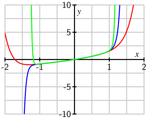
First we will plot some of the partial sums of this power series to get an idea of the interval of convergence. Let

$S_n(x) = \sum_{k=1}^{n} \frac{x^k}{k^2}$

for each $n \geq 1\text{.}$ Figure $8.6.1$ shows plots of $S_{10}(x)$ (in red), $S_{25}(x)$ (in blue), and $S_{50}(x)$ (in green).

Figure $8.6.1$ . Graphs of some partial sums of the power series $\sum_{k=1}^{\infty} \frac{x^k}{k^2}\text{.}$

The behavior of $S_{50}$ in particular suggests that $f(x)$ appears to be converging to a particular curve on the interval $(-1,1)\text{,}$ while growing without bound outside of that interval. Thus, the interval of convergence might be $-1 \lt x \lt 1\text{.}$ To verify our conjecture, we apply the Ratio Test. Now,

$a_k = \frac{x^k}{k^2}\text{,}$

$<span class="katex"><math xmlns="http://www.w3.org/1998/Math/MathML" display="block"><semantics><mtable rowspacing="0.25em" columnalign="right left" columnspacing="0em"><mtr><mtd><mstyle scriptlevel="0" displaystyle="true"><mrow><munder><mrow><mi>lim</mi><mo>⁡</mo></mrow><mrow><mi>k</mi><mo>→</mo><mi mathvariant="normal">∞</mi></mrow></munder><mfrac><mrow><mo fence="true">∣</mo><msub><mi>a</mi><mrow><mi>k</mi><mo>+</mo><mn>1</mn></mrow></msub><mo fence="true">∣</mo></mrow><mrow><mo fence="true">∣</mo><msub><mi>a</mi><mi>k</mi></msub><mo fence="true">∣</mo></mrow></mfrac></mrow></mstyle></mtd><mtd><mstyle scriptlevel="0" displaystyle="true"><mrow><mrow></mrow><mo>=</mo><munder><mrow><mi>lim</mi><mo>⁡</mo></mrow><mrow><mi>k</mi><mo>→</mo><mi mathvariant="normal">∞</mi></mrow></munder><mfrac><mfrac><mrow><mi mathvariant="normal">∣</mi><mi>x</mi><msup><mi mathvariant="normal">∣</mi><mrow><mi>k</mi><mo>+</mo><mn>1</mn></mrow></msup></mrow><mrow><mo stretchy="false">(</mo><mi>k</mi><mo>+</mo><mn>1</mn><msup><mo stretchy="false">)</mo><mn>2</mn></msup></mrow></mfrac><mfrac><mrow><mi mathvariant="normal">∣</mi><mi>x</mi><msup><mi mathvariant="normal">∣</mi><mi>k</mi></msup></mrow><msup><mi>k</mi><mn>2</mn></msup></mfrac></mfrac></mrow></mstyle></mtd></mtr><mtr><mtd><mstyle scriptlevel="0" displaystyle="true"><mrow></mrow></mstyle></mtd><mtd><mstyle scriptlevel="0" displaystyle="true"><mrow><mrow></mrow><mo>=</mo><munder><mrow><mi>lim</mi><mo>⁡</mo></mrow><mrow><mi>k</mi><mo>→</mo><mi mathvariant="normal">∞</mi></mrow></munder><mi mathvariant="normal">∣</mi><mi>x</mi><mi mathvariant="normal">∣</mi><msup><mrow><mo fence="true">(</mo><mfrac><mi>k</mi><mrow><mi>k</mi><mo>+</mo><mn>1</mn></mrow></mfrac><mo fence="true">)</mo></mrow><mn>2</mn></msup></mrow></mstyle></mtd></mtr><mtr><mtd><mstyle scriptlevel="0" displaystyle="true"><mrow></mrow></mstyle></mtd><mtd><mstyle scriptlevel="0" displaystyle="true"><mrow><mrow></mrow><mo>=</mo><mi mathvariant="normal">∣</mi><mi>x</mi><mi mathvariant="normal">∣</mi><munder><mrow><mi>lim</mi><mo>⁡</mo></mrow><mrow><mi>k</mi><mo>→</mo><mi mathvariant="normal">∞</mi></mrow></munder><msup><mrow><mo fence="true">(</mo><mfrac><mi>k</mi><mrow><mi>k</mi><mo>+</mo><mn>1</mn></mrow></mfrac><mo fence="true">)</mo></mrow><mn>2</mn></msup></mrow></mstyle></mtd></mtr><mtr><mtd><mstyle scriptlevel="0" displaystyle="true"><mrow></mrow></mstyle></mtd><mtd><mstyle scriptlevel="0" displaystyle="true"><mrow><mrow></mrow><mo>=</mo><mi mathvariant="normal">∣</mi><mi>x</mi><mi mathvariant="normal">∣</mi><mtext>.</mtext></mrow></mstyle></mtd></mtr></mtable><annotation encoding="application/x-tex">\begin{align*} \lim_{k \to \infty} \frac{\left| a_{k+1} \right|}{ \left| a_k \right|} & = \lim_{k \to \infty} \frac{ \frac{|x|^{k+1}}{(k+1)^2} }{ \frac{| x|^{k}}{k^2} }\\[4pt] & = \lim_{k \to \infty} |x| \left(\frac{k}{k+1}\right)^2\\[4pt] & = |x| \lim_{k \to \infty} \left(\frac{k}{k+1}\right)^2\\[4pt] & = |x|\text{.} \end{align*}</annotation></semantics></math></span>$

Therefore, the Ratio Test tells us that $f(x)$ converges absolutely when $| x | \lt 1$ and diverges when $| x | \gt 1\text{.}$ Because the Ratio Test is inconclusive when $|x| = 1\text{,}$ we need to check $x = 1$ and $x = -1$ individually.

When $x = 1\text{,}$ observe that

$f(1) = \sum_{k=1}^{\infty} \frac{1}{k^2}\text{.}$

This is a $p$ -series with $p \gt 1\text{,}$ which we know converges. When $x = -1\text{,}$ we have

$f(-1) = \sum_{k=1}^{\infty} \frac{(-1)^k}{k^2}\text{.}$

This is an alternating series, and since the sequence $\left\{ \frac{1}{n^2} \right\}$ decreases to 0, the power series converges by the Alternating Series Test. Thus, the interval of convergence of this power series is $-1 \le x \le 1\text{.}$

Activity $8.6.2$

Determine the interval of convergence of each power series.

$\displaystyle \sum_{k=1}^{\infty} \frac{(x-1)^k}{3k}$
$\displaystyle \sum_{k=1}^{\infty} kx^k$
$\displaystyle \sum_{k=1}^{\infty} \frac{k^2(x+1)^k}{4^k}$
$\displaystyle \sum_{k=1}^{\infty} \frac{x^k}{(2k)!}$
$\displaystyle \sum_{k=1}^{\infty} k!x^k$

Manipulating Power Series

We know power series expansions for important functions such as $\sin(x)$ and $e^x\text{.}$ Often, we can use a known power series expansion to find a power series for a different, but related, function. The next activity demonstrates one way to do this.

Activity $8.6.3$

Our goal in this activity is to find a power series expansion for $f(x) = \frac{1}{1+x^2}$ centered at $x=0\text{.}$

While we could use the methods of Section 8.5 and differentiate $f(x) = \frac{1}{1+x^2}$ several times to look for patterns and find the Taylor series for $f(x)\text{,}$ we seek an alternate approach because of how complicated the derivatives of $f(x)$ quickly become.

What is the Taylor series expansion for $g(x) = \frac{1}{1-x}\text{?}$ What is the interval of convergence of this series?
How is $g(-x^2)$ related to $f(x)\text{?}$ Explain, and hence substitute $-x^2$ for $x$ in the power series expansion for $g(x)\text{.}$ Given the relationship between $g(-x^2)$ and $f(x)\text{,}$ how is the resulting series related to $f(x)\text{?}$
For which values of $x$ will this power series expansion for $f(x)$ be valid? Why?

In a previous section we found several important Maclaurin series and their intervals of convergence. Here, we list these key functions and their corresponding expansions.

Note

$\begin{align*} \sin(x) & =\sum_{k=0}^{\infty} \frac{(-1)^k x^{2k+1}}{(2k+1)!}&\text{for}&-\infty \lt x \lt \infty\\[4pt] \cos(x) & =\sum_{k=0}^{\infty} \frac{(-1)^k x^{2k}}{(2k)!}&\text{for}&-\infty \lt x \lt \infty\\[4pt] e^x & =\sum_{k=0}^{\infty} \frac{x^{k}}{k!}&\text{for}&-\infty \lt x \lt \infty\\[4pt] \frac{1}{1-x} & =\sum_{k=0}^{\infty} x^k&\text{for}&-1 \lt x \lt 1 \end{align*}$

As we saw in Activity $8.6.3$ , we can use these known series to find other power series expansions for related functions such as $\sin(x^2)\text{,}$ $e^{5x^3}\text{,}$ and $\cos(x^5)\text{.}$

Activity $8.6.4$

Let $f$ be the function given by the power series expansion

f(x) = \sum_{k=0}^{\infty} (-1)^k \frac{x^{2k}}{(2k)!}\text{.}

Assume that we can differentiate a power series term by term, just like we can differentiate a (finite) polynomial. Use the fact that
$f(x) = 1 - \frac{x^2}{2!} + \frac{x^4}{4!} - \frac{x^6}{6!} + \cdots + (-1)^k \frac{x^{2k}}{(2k)!} + \cdots$

to find a power series expansion for $f'(x)\text{.}$
Observe that $f(x)$ and $f'(x)$ have familiar Taylor series. What familiar functions are these? What known relationship does our work demonstrate?
What is the series expansion for $f''(x)\text{?}$ What familiar function is $f''(x)\text{?}$

Our work in Activity $8.6.3$ holds more generally. The corresponding theorem, which we will not prove, states that we can differentiate a power series for a function $f$ term by term and obtain the series expansion for $f'\text{,}$ and similarly we can integrate a series expansion for a function $f$ term by term and obtain the series expansion for $\int f(x) \ dx\text{.}$ For both, the radius of convergence of the resulting series is the same as the original, though it is possible that the convergence status of the various series may differ at the endpoints. The formal statement of the Power Series Differentiation and Integration Theorem follows.

Power Series Differentiation and Integration Theorem

Suppose $f(x)$ has a power series expansion

f(x) = \sum_{k=0}^{\infty} c_kx^k

and that the series converges absolutely to $f(x)$ on the interval $-r \lt x \lt r\text{.}$ Then, the power series $\sum_{k=1}^{\infty} kc_kx^{k-1}$ obtained by differentiating the power series for $f(x)$ term by term converges absolutely to $f'(x)$ on the interval $-r \lt x \lt r\text{.}$ That is,

$f'(x) = \sum_{k=1}^{\infty} kc_kx^{k-1}, \ \text{for} \ |x| \lt r\text{.}$

Similarly, the power series $\sum_{k=0}^{\infty} c_k\frac{x^{k+1}}{k+1}$ obtained by integrating the power series for $f(x)$ term by term converges absolutely on the interval $-r \lt x \lt r\text{,}$ and

\int f(x) \ dx = \sum_{k=0}^{\infty} c_k\frac{x^{k+1}}{k+1} + C, \ \text{for} \ |x| \lt r\text{.}

This theorem validates the steps we took in Activity $8.6.4$ . It tells us that we can differentiate and integrate term by term on the interior of the interval of convergence, but it does not tell us what happens at the endpoints of this interval. We always need to check what happens at the endpoints separately. More importantly, we can use use the approach of differentiating or integrating a series term by term to find new series.

Example $8.6.3$

Find a series expansion centered at $x = 0$ for $\arctan(x)\text{,}$ as well as its interval of convergence.

Answer

While we could differentiate $\arctan(x)$ repeatedly and look for patterns in the derivative values at $x = 0$ in an attempt to find the Maclaurin series for $\arctan(x)$ from the definition, it turns out to be far easier to use a known series in an insightful way. In Activity $8.6.3$ , we found that

\frac{1}{1+x^2} = \sum_{k=0}^{\infty} (-1)^k x^{2k}

for $-1 \lt x \lt 1\text{.}$ Recall that

\frac{d}{dx} \left[ \arctan(x) \right] = \frac{1}{1+x^2}\text{,}

and therefore

\int \frac{1}{1+x^2} \ dx = \arctan(x) + C\text{.}

It follows that we can integrate the series for $\frac{1}{1+x^2}$ term by term to obtain the power series expansion for $\arctan(x)\text{.}$ Doing so, we find that

\begin{align*} \arctan(x) & = \int \left( \sum_{k=0}^{\infty} (-1)^kx^{2k} \right) \ dx\\[4pt] & = \sum_{k=0}^{\infty} \left( \int (-1)^k x^{2k} \ dx \right)\\[4pt] & = \left( \sum_{k=0}^{\infty} (-1)^k\frac{x^{2k+1}}{2k+1} \right) + C\text{.} \end{align*}

The Power Series Differentiation and Integration Theorem tells us that this equality is valid for at least $-1 \lt x \lt 1\text{.}$

To find the value of the constant $C\text{,}$ we can use the fact that $\arctan(0) = 0\text{.}$ So

0 = \arctan(0) = \left( \sum_{k=0}^{\infty} (-1)^k\frac{0^{2k+1}}{2k+1} \right) + C = C\text{,}

and we must have $C = 0\text{.}$ Therefore,

\arctan(x) = \sum_{k=0}^{\infty} (-1)^k\frac{x^{2k+1}}{2k+1}\tag{

for at least $-1 \lt x \lt 1\text{.}$

It is a straightforward exercise to check that the power series

\sum_{k=0}^{\infty} (-1)^k\frac{x^{2k+1}}{2k+1}

converges both when $x = -1$ and when $x = 1\text{;}$ in each case, we have an alternating series with terms $\frac{1}{2k+1}$ that decrease to $0\text{,}$ and thus the interval of convergence for the series expansion for $\arctan(x)$ in Equation ( $8.6.3$ ) is $-1 \le x \le 1\text{.}$

Activity $8.6.5$

Find a power series expansion for $\ln(1+x)$ centered at $x=0$ and determine its interval of convergence.

Summary

A power series is a series of the form
$\sum_{k=0}^{\infty} a_kx^k\text{.}$
We can often assume a solution to a given problem can be written as a power series, then use the information in the problem to determine the coefficients in the power series. This method allows us to approximate solutions to certain problems using partial sums of the power series; that is, we can find approximate solutions that are polynomials.
The connection between power series and Taylor series is that they are essentially the same thing: on its interval of convergence a power series is the Taylor series of its sum.

Build status · Flash Infinity AI™ is a trademark of AI-Flash Inc.. WorldClass is not affiliated with, approved or accredited by any exam board, curriculum provider or university unless a page says so.

8.6: Power Series

Motivating Questions

Preview Activity 8.6.18.6.1

Definition 8.6.18.6.1: Power Series

Example 8.6.18.6.1

Example 8.6.28.6.2

Activity 8.6.28.6.2

Manipulating Power Series

Activity 8.6.38.6.3

Note

Activity 8.6.48.6.4

Power Series Differentiation and Integration Theorem

Example 8.6.38.6.3

Activity 8.6.58.6.5

Summary

Preview Activity $8.6.1$

Definition $8.6.1$ : Power Series

Example $8.6.1$

Example $8.6.2$

Activity $8.6.2$

Activity $8.6.3$

Activity $8.6.4$

Example $8.6.3$

Activity $8.6.5$