8.5: Taylor Polynomials and Taylor Series

Taylor Polynomials

Preview Activity $8.5.1$ illustrates the first steps in the process of approximating functions with polynomials. Using this process we can approximate trigonometric, exponential, logarithmic, and other nonpolynomial functions as closely as we like (for certain values of $x$ ) with polynomials. This is extraordinarily useful in that it allows us to calculate values of these functions to whatever precision we like using only the operations of addition, subtraction, multiplication, and division, which can be easily programmed in a computer.
We next extend the approach in Preview Activity 8.5.1 to arbitrary functions at arbitrary points. Let $f$ be a function that has as many derivatives as we need at a point $x=a$. Recall that $P_1(x)$ is the tangent line to $f$ at $(a, f(a))$ and is given by the formula
$$<br /> P_1(x)=f(a)+f^{\prime}(a)(x-a) . <br />$$
$P_1(x)$ is the linear approximation to $f$ near $a$ that has the same slope and function value as $f$ at the point $x=a$.
We next want to find a quadratic approximation
$$<br /> P_2(x)=P_1(x)+c_2(x-a)^2  <br />$$
so that $P_2(x)$ more closely models $f(x)$ near $x=a$. Consider the following calculations of the values and derivatives of $P_2(x)$ :

$P_2(x)=P_1(x)+c_2(x-a)^2 \quad P_2(a)=P_1(a)=f(a)$
$P_2^{\prime}(x)=P_1^{\prime}(x)+2 c_2(x-a) \quad P_2^{\prime}(a)=P_1^{\prime}(a)=f^{\prime}(a)$
$P_2^{\prime \prime}(x)=2 c_2 \quad P_2^{\prime \prime}(a)=2 c_2$.

To make $P_2(x)$ fit $f(x)$ better than $P_1(x)$, we want $P_2(x)$ and $f(x)$ to have the same concavity at $x=a$, in addition to having the same slope and function value. That is, we want to have
$$<br /> P_2^{\prime \prime}(a)=f^{\prime \prime}(a) . <br />$$
This implies that
$$<br /> 2 c_2=f^{\prime \prime}(a) <br />$$
and thus
$$<br /> c_2=\frac{f^{\prime \prime}(a)}{2} . <br />$$
Therefore, the quadratic approximation $P_2(x)$ to $f$ centered at $x=a$ is
$$<br /> P_2(x)=f(a)+f^{\prime}(a)(x-a)+\frac{f^{\prime \prime}(a)}{2 !}(x-a)^2 . <br />$$

This approach extends naturally to polynomials of higher degree. We define polynomials
$$<br /> \begin{array}{l}<br /> P_3(x)=P_2(x)+c_3(x-a)^3, \\<br /> P_4(x)=P_3(x)+c_4(x-a)^4, \\<br /> P_5(x)=P_4(x)+c_5(x-a)^5,<br /> \end{array}  <br />$$
and in general
$$<br /> P_n(x)=P_{n-1}(x)+c_n(x-a)^n . <br />$$
The defining property of these polynomials is that for each $n, P_n(x)$ and all its first $n$ derivatives must agree with those of $f$ at $x=a$. In other words we require that
$$<br /> P_n^{(k)}(a)=f^{(k)}(a) <br />$$
for all $k$ from 0 to $n$.
To see the conditions under which this happens, suppose
$$<br /> P_n(x)=c_0+c_1(x-a)+c_2(x-a)^2+\cdots+c_n(x-a)^n . <br />$$
Then
$$<br /> \begin{array}{l}<br /> P_n^{(0)}(a)=c_0 \\<br /> P_n^{(1)}(a)=c_1 \\<br /> P_n^{(2)}(a)=2 c_2 \\<br /> P_n^{(3)}(a)=(2)(3) c_3 \\<br /> P_n^{(4)}(a)=(2)(3)(4) c_4 \\<br /> P_n^{(5)}(a)=(2)(3)(4)(5) c_5<br /> \end{array} <br />$$
and, in general,
$$<br /> P_n^{(k)}(a)=(2)(3)(4) \cdots(k-1)(k) c_k=k ! c_k . <br />$$
So having $P_n^{(k)}(a)=f^{(k)}(a)$ means that $k ! c_k=f^{(k)}(a)$ and therefore
$$<br /> c_k=\frac{f^{(k)}(a)}{k !} <br />$$
for each value of $k$. Using this expression for $c_k$, we have found the formula for the polynomial approximation of $f$ that we seek. Such a polynomial is called a Taylor polynomial.

Definition: $8.5.1$:Taylor Polynomials

The $n$th order Taylor polynomial of $f$ centered at $x=a$ is given by
$$<br /> \begin{aligned}<br /> P_n(x) &=f(a)+f^{\prime}(a)(x-a)+\frac{f^{\prime \prime}(a)}{2 !}(x-a)^2+\cdots+\frac{f^{(n)}(a)}{n !}(x-a)^n \\<br /> &=\sum_{k=0}^n \frac{f^{(k)}(a)}{k !}(x-a)^k .<br /> \end{aligned}  <br />$$
This degree $n$ polynomial approximates $f(x)$ near $x=a$ and has the property that $P_n^{(k)}(a)=f^{(k)}(a)$ for $k=0,1, \ldots, n$.

 

Example $8.5.1$

Example 8.5.1. Determine the third order Taylor polynomial for $f(x)=e^x$, as well as the general $n$th order Taylor polynomial for $f$ centered at $x=0$.

Solution

We know that $f^{\prime}(x)=e^x$ and so $f^{\prime \prime}(x)=e^x$ and $f^{\prime \prime \prime}(x)=e^x$. Thus,
$$<br /> f(0)=f^{\prime}(0)=f^{\prime \prime}(0)=f^{\prime \prime \prime}(0)=1 . <br />$$
So the third order Taylor polynomial of $f(x)=e^x$ centered at $x=0$ is
$$<br /> \begin{aligned}<br /> P_3(x) &=f(0)+f^{\prime}(0)(x-0)+\frac{f^{\prime \prime}(0)}{2 !}(x-0)^2+\frac{f^{\prime \prime \prime}(0)}{3 !}(x-0)^3 \\<br /> &=1+x+\frac{x^2}{2}+\frac{x^3}{6} .<br /> \end{aligned} <br />$$
In general, for the exponential function $f$ we have $f^{(k)}(x)=e^x$ for every positive integer $k$. Thus, the $k$ th term in the $n$th order Taylor polynomial for $f(x)$ centered at $x=0$ is
$$<br /> \frac{f^{(k)}(0)}{k !}(x-0)^k=\frac{1}{k !} x^k . <br />$$
Therefore, the $n$th order Taylor polynomial for $f(x)=e^x$ centered at $x=0$ is
$$<br /> P_n(x)=1+x+\frac{x^2}{2 !}+\cdots+\frac{1}{n !} x^n=\sum_{k=0}^n \frac{x^k}{k !} . <br />$$

Activity $8.5.2$

We have just seen that the $n$th order Taylor polynomial centered at $a=0$ for the exponential function $e^x$ is
$$<br /> \sum_{k=0}^n \frac{x^k}{k !} . <br />$$
In this activity, we determine small order Taylor polynomials for several other familiar functions, and look for general patterns.

a. Let $f(x)=\frac{1}{1-x}$.

i. Calculate the first four derivatives of $f(x)$ at $x=0$. Then find the fourth order Taylor polynomial $P_4(x)$ for $\frac{1}{1-x}$ centered at 0 .
ii. Based on your results from part (i), determine a general formula for $f^{(k)}(0)$

b. Let $f(x)=\cos (x)$.

i. Calculate the first four derivatives of $f(x)$ at $x=0$. Then find the fourth order Taylor polynomial $P_4(x)$ for $\cos (x)$ centered at 0 .
ii. Based on your results from part (i), find a general formula for $f^{(k)}(0)$. (Think about how $k$ being even or odd affects the value of the $k$ th derivative.)

c. Let $f(x)=\sin (x)$.

i. Calculate the first four derivatives of $f(x)$ at $x=0$. Then find the fourth order Taylor polynomial $P_4(x)$ for $\sin (x)$ centered at 0 .
ii. Based on your results from part (i), find a general formula for $f^{(k)}(0)$. (Think about how $k$ being even or odd affects the value of the $k$ th derivative.)

It is possible that an $n$th order Taylor polynomial is not a polynomial of degree $n$; that is, the order of the approximation can be different from the degree of the polynomial. For example, in Activity 8.5.3 we found that the second order Taylor polynomial $P_2(x)$ centered at 0 for $\sin (x)$ is $P_2(x)=x$. In this case, the second order Taylor polynomial is a degree 1 polynomial.

Taylor Series

In Activity $8.5.2$ we saw that the fourth order Taylor polynomial $P_4(x)$ for $\sin (x)$ centered at 0 is
$$<br /> P_4(x)=x-\frac{x^3}{3 !} . <br />$$
The pattern we found for the derivatives $f^{(k)}(0)$ describe the higher-order Taylor polynomials, e.g.,
$$<br /> \begin{array}{l}<br /> P_5(x)=x-\frac{x^3}{3 !}+\frac{x^5}{5 !}, \\<br /> P_7(x)=x-\frac{x^3}{3 !}+\frac{x^5}{5 !}-\frac{x^7}{7 !}, \\<br /> P_9(x)=x-\frac{x^3}{3 !}+\frac{x^5}{5 !}-\frac{x^7}{7 !}+\frac{x^9}{9 !},<br /> \end{array} <br />$$
and so on. It is instructive to consider the graphical behavior of these functions; Figure $8.5.1$ shows the graphs of a few of the Taylor polynomials centered at 0 for the sine function.

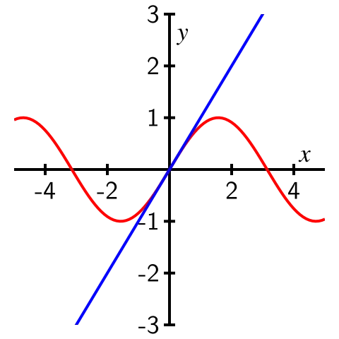
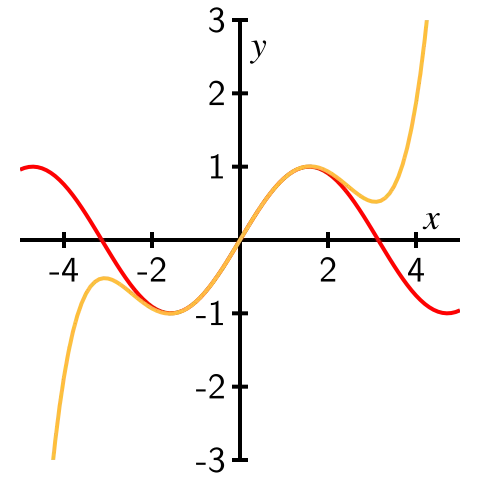
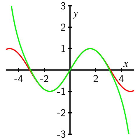
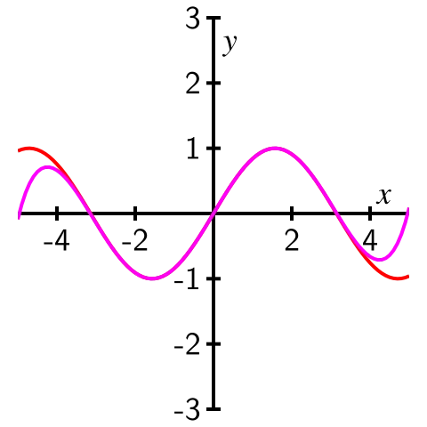
Notice that $P_1(x)$ is close to the sine function only for values of $x$ that are close to 0 , but as we increase the degree of the Taylor polynomial the Taylor polynomials provide a better fit to the graph of the sine function over larger intervals. This illustrates the general behavior of Taylor polynomials: for any sufficiently well-behaved function, the sequence $\left\{P_n(x)\right\}$ of Taylor polynomials converges to the function $f$ on larger and larger intervals (though those intervals may not necessarily increase without bound). If the Taylor polynomials ultimately converge to $f$ on its entire domain, we write

$$<br /> f(x)=\sum_{k=0}^{\infty} \frac{f^{(k)}(a)}{k !}(x-a)^k . <br />$$

Definition: $8.5.2$

 Let $f$ be a function all of whose derivatives exist at $x=a$. The Taylor series for $f$ centered at $x=a$ is the series $T_f(x)$ defined by
$$<br /> T_f(x)=\sum_{k=0}^{\infty} \frac{f^{(k)}(a)}{k !}(x-a)^k .<br />$$

In the special case where $a=0$ in Definition 8.5.3, the Taylor series is also called the Maclaurin series for $f$. From Example 8.5.1 we know the $n$th order Taylor polynomial centered at 0 for the exponential function $e^x$; thus, the Maclaurin series for $e^x$ is
$$<br /> \sum_{k=0}^{\infty} \frac{x^k}{k !} . <br />$$

Activity $8.5.3$

In Activity 8.5.2\</span> we determined small order Taylor polynomials for a few familiar functions, and also found general patterns in the derivatives evaluated at 0 . Use that information to write the Taylor series centered at 0 for the following functions.</p> <p>a. \(f(x)=\frac{1}{1-x}
b. $f(x)=\cos (x)$ (You will need to carefully consider how to indicate that many of the coefficients are 0 . Think about a general way to represent an even integer.)
c. $f(x)=\sin (x)$ (You will need to carefully consider how to indicate that many of the coefficients are 0 . Think about a general way to represent an odd integer.)
d. $f(x)=\frac{1}{1+x}$

 

Activity $8.5.4$

1. Plot the graphs of several of the Taylor polynomials centered at 0 (of order at least 5) for $e^x$ and convince yourself that these Taylor polynomials converge to $e^x$ for every value of $x$.
2. Draw the graphs of several of the Taylor polynomials centered at 0 (of order at least 6$)$ for $\cos (x)$ and convince yourself that these Taylor polynomials converge to $\cos (x)$ for every value of $x$. Write the Taylor series centered at 0 for $\cos (x)$.
3. Draw the graphs of several of the Taylor polynomials centered at 0 for $\frac{1}{1-x}$. Based on your graphs, for what values of $x$ do these Taylor polynomials appear to converge to $\frac{1}{1-x}$ ? How is this situation different from what we observe with $e^x$ and $\cos (x)$ ? In addition, write the Taylor series centered at 0 for $\frac{1}{1-x}$.

The Maclaurin series for $e^x, \sin (x), \cos (x)$, and $\frac{1}{1-x}$ will be used frequently, so we should be certain to know and recognize them well.

The Interval of Convergence of a Taylor Series

In the previous section (in Figure $8.5.1$ and Activity $8.5.4$) we observed that the Taylor polynomials centered at 0 for $e^x, \cos (x)$, and $\sin (x)$ converged to these functions for all values of $x$ in their domain, but that the Taylor polynomials centered at 0 for $\frac{1}{1-x}$ converge to $\frac{1}{1-x}$ on the interval $(-1,1)$ and diverge for all other values of $x$. So the Taylor series for a function $f(x)$ does not need to converge for all values of $x$ in the domain of $f$.
Our observations suggest two natural questions: can we determine the values of $x$ for which a given Taylor series converges? And does the Taylor series for a function $f$ actually converge to $f(x)$ ?

Example $8.5.1$

Graphical evidence suggests that the Taylor series centered at 0 for $e^x$ converges for all values of $x$. To verify this, use the Ratio Test to determine all values of $x$ for which the Taylor series
$$<br /> \sum_{k=0}^{\infty} \frac{x^k}{k !} <br />$$
converges absolutely.

Solution

Recall that the Ratio Test applies only to series of nonnegative terms. In this example, the variable $x$ may have negative values. But we are interested in absolute convergence, so we apply the Ratio Test to the series
$$<br /> \sum_{k=0}^{\infty}\left|\frac{x^k}{k !}\right|=\sum_{k=0}^{\infty} \frac{|x|^k}{k !} . <br />$$
Now, observe that
$$<br /> \begin{aligned}<br /> \lim _{k \rightarrow \infty} \frac{a_{k+1}}{a_k} &=\lim _{k \rightarrow \infty} \frac{\frac{|x|^{k+1}}{(k+1) !}}{\frac{|x|^k}{k}} \\<br /> &=\lim _{k \rightarrow \infty} \frac{|x|^{k+1} k !}{|x|^k(k+1) !} \\<br /> &=\lim _{k \rightarrow \infty} \frac{|x|}{k+1} \\<br /> &=0<br /> \end{aligned} <br />$$
for any value of $x$. So the Taylor series ($8.5.4$) converges absolutely for every value of $x$, and thus converges for every value of $x$.

One question still remains: while the Taylor series for $e^x$ converges for all $x$, what we have done does not tell us that this Taylor series actually converges to $e^x$ for each $x$. We'll return to this question when we consider the error in a Taylor approximation near the end of this section.
We can apply the main idea from Example 8.5.4 in general. To determine the values of $x$ for which a Taylor series
$$<br /> \sum_{k=0}^{\infty} c_k(x-a)^k <br />$$
centered at $x=a$ will converge, we apply the Ratio Test with $a_k=\left|c_k(x-a)^k\right|$. The series converges if $\lim _{k \rightarrow \infty} \frac{a_{k+1}}{a_k}<1$.
Observe that
$$<br /> \frac{a_{k+1}}{a_k}=|x-a| \frac{\left|c_{k+1}\right|}{\left|c_k\right|} <br />$$
so when we apply the Ratio Test, we get
$$<br /> \lim _{k \rightarrow \infty} \frac{a_{k+1}}{a_k}=\lim _{k \rightarrow \infty}|x-a| \frac{\left|c_{k+1}\right|}{\left|c_k\right|} . <br />$$
Note suppose that
$$<br /> \lim _{k \rightarrow \infty} \frac{\left|c_{k+1}\right|}{\left|c_k\right|}=L <br />$$

so that
$$<br /> \lim _{k \rightarrow \infty} \frac{a_{k+1}}{a_k}=|x-a| \cdot L . <br />$$
There are three possibilities for $L: L$ can be 0 , it can be a finite positive value, or it can be infinite. Based on this value of $L$, we can determine for which values of $x$ the original Taylor series converges.

• If $L=0$, then the Taylor series converges on $(-\infty, \infty)$.
• If $L$ is infinite, then the Taylor series converges only at $x=a$.
• If $L$ is finite and nonzero, then the Taylor series converges absolutely for all $x$ that satisfy
  $$|x-a| \cdot L<1$$
  or for all $x$ such that
  $$|x-a|<\frac{1}{L},$$ 
  which is the interval
  $$\left(a-\frac{1}{L}, a+\frac{1}{L}\right).$$ 

Because the Ratio Test is inconclusive when the $|x-a| \cdot L=1$, the endpoints $a \pm \frac{1}{L}$ have to be checked separately.

It is important to notice that the set of $x$ values at which a Taylor series converges is always an interval centered at $x=a$. For this reason, the set on which a Taylor series converges is called the interval of convergence. Half the length of the interval of convergence is called the radius of convergence. If the interval of convergence of a Taylor series is infinite, then we say that the radius of convergence is infinite.

Activity $8.5.4$

1. Use the Ratio Test to explicitly determine the interval of convergence of the Taylor series for $f(x)=\frac{1}{1-x}$ centered at $x=0$.
2. Use the Ratio Test to explicitly determine the interval of convergence of the Taylor series for $f(x)=\cos (x)$ centered at $x=0$.
3. Use the Ratio Test to explicitly determine the interval of convergence of the Taylor series for $f(x)=\sin (x)$ centered at $x=0$.

The Ratio Test allows us to determine the set of $x$ values for which a Taylor series converges absolutely. However, just because a Taylor series for a function $f$ converges, we cannot be certain that the Taylor series actually converges to $f(x)$. To show why and where a Taylor series does in fact converge to the function $f$, we next consider the error that is present in Taylor polynomials.

Error Approximations for Taylor Polynomials

We now know how to find Taylor polynomials for functions such as $\sin (x)$, and how to determine the interval of convergence of the corresponding Taylor series. We next develop an error bound that will tell us how well an $n$th order Taylor polynomial $P_n(x)$ approximates its generating function $f(x)$. This error bound will also allow us to determine whether a Taylor series on its interval of convergence actually equals the function $f$ from which the Taylor series is derived. Finally, we will be able to use the error bound to determine the order of the Taylor polynomial $P_n(x)$ that we will ensure that $P_n(x)$ approximates $f(x)$ to the desired degree of accuracy.

For this argument, we assume throughout that we center our approximations at 0 (but a similar argument holds for approximations centered at $a$ ). We define the exact error, $E_n(x)$, that results from approximating $f(x)$ with $P_n(x)$ by
$$<br /> E_n(x)=f(x)-P_n(x) . <br />$$
We are particularly interested in $\left|E_n(x)\right|$, the distance between $P_n$ and $f$.
Because
$$<br /> P_n^{(k)}(0)=f^{(k)}(0) <br />$$
for $0 \leq k \leq n$, we know that
$$<br /> E_n^{(k)}(0)=0 <br />$$
for $0 \leq k \leq n$. Furthermore, since $P_n(x)$ is a polynomial of degree less than or equal to $n$, we know that
$$<br /> P_n^{(n+1)}(x)=0 . <br />$$
Thus, since $E_n^{(n+1)}(x)=f^{(n+1)}(x)-P_n^{(n+1)}(x)$, it follows that
$$<br /> E_n^{(n+1)}(x)=f^{(n+1)}(x) <br />$$
for all $x$.

Suppose that we want to approximate $f(x)$ at a number $c$ close to 0 using $P_n(c)$. If we assume $\left|f^{(n+1)}(t)\right|$ is bounded by some number $M$ on $[0, c]$, so that
$$<br /> \left|f^{(n+1)}(t)\right| \leq M <br />$$
for all $0 \leq t \leq c$, then we can say that
$$<br /> \left|E_n^{(n+1)}(t)\right|=\left|f^{(n+1)}(t)\right| \leq M <br />$$
for all $t$ between 0 and $c$. Equivalently,
$$<br /> -M \leq E_n^{(n+1)}(t) \leq M <br />$$
on $[0, c]$. Next, we integrate the three terms in Inequality $8.5.5$ from $t=0$ to $t=x$, and thus find that

$$<br /> \int_0^x-M d t \leq \int_0^x E_n^{(n+1)}(t) d t \leq \int_0^x M d t <br />$$
for every value of $x$ in $[0, c]$. Since $E_n^{(n)}(0)=0$, the First FTC tells us that
$$<br /> -M x \leq E_n^{(n)}(x) \leq M x <br />$$
for every $x$ in $[0, c]$.
Integrating this last inequality, we obtain
$$<br /> \int_0^x-M t d t \leq \int_0^x E_n^{(n)}(t) d t \leq \int_0^x M t_{-} d t <br />$$
and thus
$$<br /> -M \frac{x^2}{2} \leq E_n^{(n-1)}(x) \leq M \frac{x^2}{2} <br />$$
for all $x$ in $[0, c]$.
Integrating $n$ times, we arrive at
$$<br /> -M \frac{x^{n+1}}{(n+1) !} \leq E_n(x) \leq M \frac{x^{n+1}}{(n+1) !} <br />$$
for all $x$ in $[0, c]$. This enables us to conclude that
$$<br /> \left|E_n(x)\right| \leq M \frac{|x|^{n+1}}{(n+1) !} <br />$$
for all $x$ in $[0, c]$, and we have found a bound on the approximation's error, $E_n$.
Our work above was based on the approximation centered at $a=0$; the argument may be generalized to hold for any value of $a$, which results in the following theorem.

Definition: $8.5.3$: The Lagrange Error Bound 

The Lagrange Error Bound for $P_n(x)$.

Let $f$ be a continuous function with $n+1$ continuous derivatives. Suppose that $M$ is a positive real number such that $\left|f^{(n+1)}(x)\right| \leq M$ on the interval $[a, c]$. If $P_n(x)$ is the $n$th order Taylor polynomial for $f(x)$ centered at $x=a$, then
$$<br /> \left|P_n(c)-f(c)\right| \leq M \frac{|c-a|^{n+1}}{(n+1) !} . <br />$$

We can use this error bound to tell us important information about Taylor polynomials and Taylor series, as we see in the following examples and activities.

Example $8.5.5$

Determine how well the 10th order Taylor polynomial $P_{10}(x)$ for $\sin (x)$, centered at 0 , approximates $\sin (2)$.

Solution

To answer this question we use $f(x)=\sin (x), c=2, a=0$, and $n=10$ in the Lagrange error bound formula. We also need to find an appropriate value for $M$. Note that the derivatives of $f(x)=\sin (x)$ are all equal to $\pm \sin (x)$ or $\pm \cos (x)$. Thus,
$$<br /> \left|f^{(n+1)}(x)\right| \leq 1 <br />$$
for any $n$ and $x$. Therefore, we can choose $M$ to be 1 . Then
$$<br /> \left|P_{10}(2)-f(2)\right| \leq(1) \frac{|2-0|^{11}}{(11) !}=\frac{2^{11}}{(11) !} \approx 0.00005130671797 . <br />$$
So $P_{10}(2)$ approximates $\sin (2)$ to within at most $0.00005130671797$. A computer algebra system tells us that
$$<br /> P_{10}(2) \approx 0.9093474427 \text { and } \sin (2) \approx 0.9092974268 <br />$$
with an actual difference of about $0.0000500159$.

 

Activity $8.5.6$

Let $P_n(x)$ be the $n$th order Taylor polynomial for $\sin (x)$ centered at $x=0$. Determine how large we need to choose $n$ so that $P_n(2)$ approximates $\sin (2)$ to 20 decimal places.

 

Example $8.5.6$

Show that the Taylor series for $\sin (x)$ actually converges to $\sin (x)$ for all $x$.

Solution

Recall from the previous example that since $f(x)=\sin (x)$, we know
$$<br /> \left|f^{(n+1)}(x)\right| \leq 1 <br />$$
for any $n$ and $x$. This allows us to choose $M=1$ in the Lagrange error bound formula. Thus,
$$<br /> \left|P_n(x)-\sin (x)\right| \leq \frac{|x|^{n+1}}{(n+1) !} <br />$$
for every $x$.
We showed in earlier work that the Taylor series $\sum_{k=0}^{\infty} \frac{x^k}{k !}$ converges for every value of $x$. Because the terms of any convergent series must approach zero, it follows that
$$<br /> \lim _{n \rightarrow \infty} \frac{x^{n+1}}{(n+1) !}=0  <br />$$
for every value of $x$. Thus, taking the limit as $n \rightarrow \infty$ in the inequality $8.5.6$, it follows that
$$<br /> \lim _{n \rightarrow \infty}\left|P_n(x)-\sin (x)\right|=0 . <br />$$
As a result, we can now write
$$<br /> \sin (x)=\sum_{n=0}^{\infty} \frac{(-1)^n x^{2 n+1}}{(2 n+1) !} <br />$$
for every real number $x$.

Activity $8.5.7$

1. Show that the Taylor series centered at 0 for $\cos (x)$ converges to $\cos (x)$ for every real number $x$.
2. Next we consider the Taylor series for $e^x$.

 

1. Show that the Taylor series centered at 0 for $e^x$ converges to $e^x$ for every nonnegative value of $x$.
2. Show that the Taylor series centered at 0 for $e^x$ converges to $e^x$ for every negative value of $x$.
3. Explain why the Taylor series centered at 0 for $e^x$ converges to $e^x$ for every real number $x$. Recall that we earlier showed that the Taylor series centered at 0 for $e^x$ converges for all $x$, and we have now completed the argument that the Taylor series for $e^x$ actually converges to $e^x$ for all $x$.

 

3. Let $P_n(x)$ be the $n$th order Taylor polynomial for $e^x$ centered at 0 . Find a value of $n$ so that $P_n(5)$ approximates $e^5$ correct to 8 decimal places.

Summary

• We can use Taylor polynomials to approximate functions. This allows us to approximate values of functions using only addition, subtraction, multiplication, and division of real numbers. The $n$th order Taylor polynomial centered at $x=a$ of a function $f$ is
  $$\begin{aligned} P_n(x) &=f(a)+f^{\prime}(a)(x-a)+\frac{f^{\prime \prime}(a)}{2 !}(x-a)^2+\cdots+\frac{f^{(n)}(a)}{n !}(x-a)^n \\&=\sum_{k=0}^n \frac{f^{(k)}(a)}{k !}(x-a)^k .\end{aligned}$$ 
• The Taylor series centered at $x=a$ for a function $f$ is
  $$\sum_{k=0}^{\infty} \frac{f^{(k)}(a)}{k !}(x-a)^k .$$
  The $n$th order Taylor polynomial centered at $a$ for $f$ is the $n$th partial sum of its Taylor series centered at $a$. So the $n$th order Taylor polynomial for a function $f$ is an approximation to $f$ on the interval where the Taylor series converges; for the values of $x$ for which the Taylor series converges to $f$ we write
  $$f(x)=\sum_{k=0}^{\infty} \frac{f^{(k)}(a)}{k !}(x-a)^k .$$
• The Lagrange Error Bound shows us how to determine the accuracy in using a Taylor polynomial to approximate a function. More specifically, if $P_n(x)$ is the $n$th order Taylor polynomial for $f$ centered at $x=a$ and if $M$ is an upper bound for $\left|f^{(n+1)}(x)\right|$ on the interval $[a, c]$, then
  $$\left|P_n(c)-f(c)\right| \leq M \frac{|c-a|^{n+1}}{(n+1) !} .$$