1.1: How do we Measure Velocity?

Position and average velocity

Any moving object has a position that can be considered a function of time. When the motion is along a straight line, the position is given by a single variable, which we denote by $s(t)\text{.}$ For example, $s(t)$ might give the mile marker of a car traveling on a straight highway at time $t$ in hours. Similarly, the function $s$ described in Preview Activity $1.1.1$ is a position function, where position is measured vertically relative to the ground.

On any time interval, a moving object also has an average velocity. For example, to compute a car's average velocity we divide the number of miles traveled by the time elapsed, which gives the velocity in miles per hour. Similarly, the value of $AV_{[0.5,1]}$ in Preview Activity $1.1.1$ gave the average velocity of the ball on the time interval $[0.5,1]\text{,}$ measured in feet per second.

In general, we make the following definition:

Average Velocity

For an object moving in a straight line with position function $s(t)\text{,}$ the average velocity of the object on the interval from $t = a$ to $t = b$, denoted $AV_{[a,b]}\text{,}$ is given by the formula

$$AV_{[a,b]} = \frac{s(b)-s(a)}{b-a}\text{.}$$

Note well: the units on $AV_{[a,b]}$ are “units of $s$ per unit of $t\text{,}$” such as “miles per hour” or “feet per second.”

Activity $1.1.2$

The following questions concern the position function given by $s(t) = 64 - 16(t-1)^2\text{,}$ considered in Preview Activity $1.1.1$.

1. Compute the average velocity of the ball on each of the following time intervals: $[0.4,0.8]\text{,}$ $[0.7,0.8]\text{,}$ $[0.79, 0.8]\text{,}$ $[0.799,0.8]\text{,}$ $[0.8,1.2]\text{,}$ $[0.8,0.9]\text{,}$ $[0.8,0.81]\text{,}$ $[0.8,0.801]\text{.}$ Include units for each value.
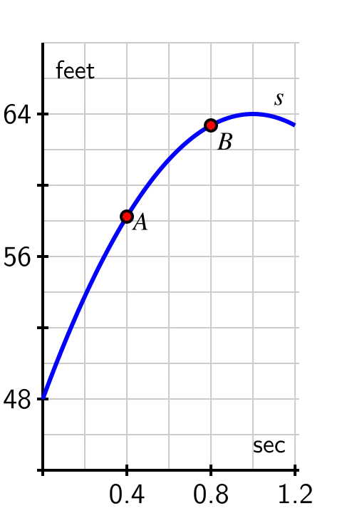
2. On the graph provided in Figure $1.1.1$, sketch the line that passes through the points $A=(0.4, s(0.4))$ and $B=(0.8, s(0.8))\text{.}$ What is the meaning of the slope of this line? In light of this meaning, what is a geometric way to interpret each of the values computed in the preceding question?
3. Use a graphing utility to plot the graph of $s(t) = 64 - 16(t-1)^2$ on an interval containing the value $t = 0.8\text{.}$ Then, zoom in repeatedly on the point $(0.8, s(0.8))\text{.}$ What do you observe about how the graph appears as you view it more and more closely?
4. What do you conjecture is the velocity of the ball at the instant $t = 0.8\text{?}$ Why?

Instantaneous Velocity

Whether we are driving a car, riding a bike, or throwing a ball, we have an intuitive sense that a moving object has a velocity at any given moment -- a number that measures how fast the object is moving right now. For instance, a car's speedometer tells the driver the car's velocity at any given instant. In fact, the velocity on a speedometer is really an average velocity that is computed over a very small time interval. If we let the time interval over which average velocity is computed become shorter and shorter, we can progress from average velocity to instantaneous velocity.

Informally, we define the instantaneous velocity of a moving object at time $t = a$ to be the value that the average velocity approaches as we take smaller and smaller intervals of time containing $t = a\text{.}$ We will develop a more formal definition of instantaneous velocity soon, and this definition will be the foundation of much of our work in calculus. For now, it is fine to think of instantaneous velocity as follows: take average velocities on smaller and smaller time intervals around a specific point. If those average velocities approach a single number, then that number will be the instantaneous velocity at that point.

Activity $1.1.3$

Each of the following questions concern $s(t) = 64 - 16(t-1)^2\text{,}$ the position function from Preview Activity $1.1.1$.

1. Compute the average velocity of the ball on the time interval $[1.5,2]\text{.}$ What is different between this value and the average velocity on the interval $[0,0.5]\text{?}$
2. Use appropriate computing technology to estimate the instantaneous velocity of the ball at $t = 1.5\text{.}$ Likewise, estimate the instantaneous velocity of the ball at $t = 2\text{.}$ Which value is greater?
3. How is the sign of the instantaneous velocity of the ball related to its behavior at a given point in time? That is, what does positive instantaneous velocity tell you the ball is doing? Negative instantaneous velocity?
4. Without doing any computations, what do you expect to be the instantaneous velocity of the ball at $t = 1\text{?}$ Why?

At this point we have started to see a close connection between average velocity and instantaneous velocity. Each is connected not only to the physical behavior of the moving object but also to the geometric behavior of the graph of the position function. We are interested in computing average velocities on the interval $[a,b]$ for smaller and smaller intervals. In order to make the link between average and instantaneous velocity more formal, think of the value $b$ as $b = a + h\text{,}$ where $h$ is a small (non-zero) number that is allowed to vary. Then the average velocity of the object on the interval $[a,a+h]$ is

$$AV_{[a,a+h]} = \frac{s(a+h)-s(a)}{h}\text{,}$$

with the denominator being simply $h$ because $(a+h) - a = h\text{.}$ Note that when $h \lt 0\text{,}$ $AV_{[a,a+h]}$ measures the average velocity on the interval $[a+h,a]\text{.}$

To find the instantaneous velocity at $t = a\text{,}$ we investigate what happens as the value of $h$ approaches zero.

Example $1.1.2$. Computing instantaneous velocity for a falling ball

The position function for a falling ball is given by $s(t) = 16 - 16t^2$ (where $s$ is measured in feet and $t$ in seconds).

1. Find an expression for the average velocity of the ball on a time interval of the form $[0.5, 0.5+h]$ where $-0.5 \lt h \lt 0.5$ and $h \ne 0\text{.}$
2. Use this expression to compute the average velocity on $[0.5,0.75]$ and $[0.4,0.5]\text{.}$
3. Make a conjecture about the instantaneous velocity at $t = 0.5\text{.}$

Answer

a. We make the assumptions that $-0.5 \lt h \lt 0.5$ and $h \ne 0$ because $h$ cannot be zero (otherwise there is no interval on which to compute average velocity) and because the function only makes sense on the time interval $0 \le t \le 1\text{,}$ as this is the duration of time during which the ball is falling. We want to compute and simplify

$$AV_{[0.5, 0.5+h]} = \frac{s(0.5+h) - s(0.5)}{(0.5+h) - 0.5}\text{.}$$

We start by finding $s(0.5+h)\text{.}$ To do so, we follow the rule that defines the function $s\text{.}$

$$\begin{align*} s(0.5+h) & = 16 - 16(0.5 + h)^2\\[4pt] & = 16 - 16(0.25 + h + h^2)\\[4pt] & = 16 - 4 - 16h - 16h^2\\[4pt] & = 12 - 16h - 16h^2\text{.} \end{align*}$$

Now, returning to our computation of the average velocity, we find that

$$\begin{align*} AV_{[0.5, 0.5+h]} & = \frac{s(0.5+h) - s(0.5)}{(0.5+h) - 0.5}\\[4pt] & = \frac{(12 - 16h - 16h^2) - (16 - 16(0.5)^2)}{0.5 + h - 0.5}\\[4pt] & = \frac{12 - 16h - 16h^2 - 12}{h}\\[4pt] & = \frac{-16h - 16h^2}{h}\text{.} \end{align*}$$

At this point, we note two things: first, the expression for average velocity clearly depends on $h\text{,}$ which it must, since as $h$ changes the average velocity will change. Further, we note that since $h$ can never equal zero, we may remove the common factor of $h$ from the numerator and denominator. It follows that

$$AV_{[0.5, 0.5+h]} = -16 - 16h\text{.}$$

b. From this expression we can compute the average for any small positive or negative value of $h\text{.}$ For instance, to obtain the average velocity on $[0.5,0.75]\text{,}$ we let $h = 0.25\text{,}$ and the average velocity is $-16 - 16(0.25) = -20$ ft/sec. To get the average velocity on $[0.4, 0.5]\text{,}$ we let $h = -0.1\text{,}$ and compute the average velocity as

$$-16 - 16(-0.1) = -14.4\ \text{ft/sec}\text{.}$$

c. We can even explore what happens to $AV_{[0.5, 0.5+h]}$ as $h$ gets closer and closer to zero. As $h$ approaches zero, $-16h$ will also approach zero, so it appears that the instantaneous velocity of the ball at $t = 0.5$ should be $-16$ ft/sec.

Activity $1.1.4$

For the function given by $s(t) = 64 - 16(t-1)^2$ from Preview Activity $1.1.1$, find the most simplified expression you can for the average velocity of the ball on the interval $[2, 2+h]\text{.}$ Use your result to compute the average velocity on $[1.5,2]$ and to estimate the instantaneous velocity at $t = 2\text{.}$ Finally, compare your earlier work in Activity $1.1.2$.

Summary

• For an object moving in a straight line with position function $s(t)\text{,}$ the average velocity of the object on the interval from $t = a$ to $t = b$, denoted $AV_{[a,b]}\text{,}$ is given by the formula

  $$AV_{[a,b]} = \frac{s(b)-s(a)}{b-a}\text{.}$$

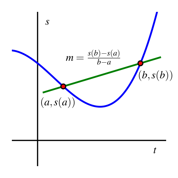
• The average velocity on $[a,b]$ can be viewed geometrically as the slope of the line between the points $(a,s(a))$ and $(b,s(b))$ on the graph of $y = s(t)\text{,}$ as shown in Figure $1.1.2$.

• Given a moving object whose position at time $t$ is given by a function $s\text{,}$ the average velocity of the object on the time interval $[a,b]$ is given by $AV_{[a,b]} = \frac{s(b) - s(a)}{b-a}\text{.}$ Viewing the interval $[a,b]$ as having the form $[a,a+h]\text{,}$ we equivalently compute average velocity by the formula $AV_{[a,a+h]} = \frac{s(a+h) - s(a)}{h}\text{.}$
• The instantaneous velocity of a moving object at a fixed time is estimated by considering average velocities on shorter and shorter time intervals that contain the instant of interest.