Chapter 5 introduced a framework for statistical inference based on confidence intervals and hypotheses using the normal distribution for sample proportions. In this chapter, we encounter several new point estimates and a couple new distributions. In each case, the inference ideas remain the same: determine which point estimate or test statistic is useful, identify an appropriate distribution for the point estimate or test statistic, and apply the ideas of inference.

One-sample means with the

\boldsymbol{t}

-distribution

to how we can model the behavior of the sample proportion $\hat{p}$ using a normal distribution, the sample mean $\bar{x}$ can also be modeled using a normal distribution when certain conditions are met.

However, we’ll soon learn that a new distribution, called the $t$ -distribution, tends to be more useful when working with the sample mean. We’ll first learn about this new distribution, then we’ll use it to construct confidence intervals and conduct hypothesis tests for the mean.

The sampling distribution of $\boldsymbol{\bar{x}}$

The sample mean tends to follow a normal distribution centered at the population mean, $\mu$ , when certain conditions are met. Additionally, we can compute a standard error for the sample mean using the population standard deviation $\sigma$ and the sample size $n$ .

Central Limit Theorem for the sample mean

When we collect a sufficiently large sample of $n$ independent observations from a population with mean $\mu$ and standard deviation $\sigma$ , the sampling distribution of $\bar{x}$ will be nearly normal with $\begin{aligned} &\text{Mean}=\mu &&\text{Standard Error }(SE) = \frac{\sigma}{\sqrt{n}} \end{aligned}$

diving into confidence intervals and hypothesis tests using $\bar{x}$ , we first need to cover two topics:

When we modeled $\hat{p}$ using the normal distribution, certain conditions had to be satisfied. The conditions for working with $\bar{x}$ are a little more complex, and we’ll spend Section 7 discussing how to check conditions for inference.
The standard error is dependent on the population standard deviation, $\sigma$ . However, we rarely know $\sigma$ , and instead we must estimate it. Because this estimation is itself imperfect, we use a new distribution called the $t$ -distribution to fix this problem, which we discuss in Section 7.1.

Evaluating the two conditions required for modeling $\boldsymbol{\bar{x}}$

conditions are required to apply the Central Limit Theorem for a sample mean $\bar{x}$ :

Independence.: The sample observations must be independent, The most common way to satisfy this condition is when the sample is a simple random sample from the population. If the data come from a random process, analogous to rolling a die, this would also satisfy the independence condition.
Normality.: When a sample is small, we also require that the sample observations come from a normally distributed population. We can relax this condition more and more for larger and larger sample sizes. This condition is obviously vague, making it difficult to evaluate, so next we introduce a couple rules of thumb to make checking this condition easier.

Rules of thumb: how to perform the normality check

There is no perfect way to check the normality condition, so instead we use two rules of thumb:

$\mathbf{n < 30}$ :: If the sample size $n$ is less than 30 and there are no clear outliers in the data, then we typically assume the data come from a nearly normal distribution to satisfy the condition.
$\mathbf{n \geq 30}$ :: If the sample size $n$ is at least 30 and there are no particularly extreme outliers, then we typically assume the sampling distribution of $\bar{x}$ is nearly normal, even if the underlying distribution of individual observations is not.

In this first course in statistics, you aren’t expected to develop perfect judgement on the normality condition. However, you are expected to be able to handle clear cut cases based on the rules of thumb.¹

Example 7.1

Consider the following two plots that come from simple random samples from different populations. Their sample sizes are $n_1 = 15$ and $n_2 = 50$ .

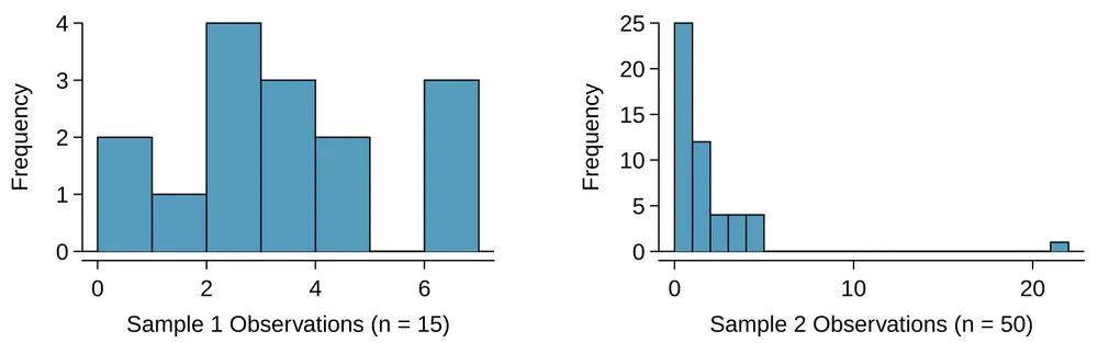
Are the independence and normality conditions met in each case?

Each samples is from a simple random sample of its respective population, so the independence condition is satisfied. Let’s next check the normality condition for each using the rule of thumb.

The first sample has fewer than 30 observations, so we are watching for any clear outliers. None are present; while there is a small gap in the histogram between 5 and 6, this gap is small and 20% of the observations in this small sample are represented in that far right bar of the histogram, so we can hardly call these clear outliers. With no clear outliers, the normality condition is reasonably met.

The second sample has a sample size greater than 30 and includes an outlier that appears to be roughly 5 times further from the center of the distribution than the next furthest observation. This is an example of a particularly extreme outlier, so the normality condition would not be satisfied.

In practice, it’s typical to also do a mental check to evaluate whether we have reason to believe the underlying population would have moderate skew (if $n < 30$ ) or have particularly extreme outliers ( $n \geq 30$ ) beyond what we observe in the data. For example, consider the number of followers for each individual account on Twitter, and then imagine this distribution. The large majority of accounts have built up a couple thousand followers or fewer, while a relatively tiny fraction have amassed tens of millions of followers, meaning the distribution is extremely skewed. When we know the data come from such an extremely skewed distribution, it takes some effort to understand what sample size is large enough for the normality condition to be satisfied.

Introducing the $\boldsymbol{t}$ -distribution

In practice, we cannot directly calculate the standard error for $\bar{x}$ since we do not know the population standard deviation, $\sigma$ . We encountered a similar issue when computing the standard error for a sample proportion, which relied on the population proportion, $p$ . Our solution in the proportion context was to use sample value in place of the population value when computing the standard error. We’ll employ a similar strategy for computing the standard error of $\bar{x}$ , using the sample standard deviation $s$ in place of $\sigma$ : $\begin{aligned} SE = \frac{\sigma}{\sqrt{n}} \approx \frac{s}{\sqrt{n}} \end{aligned}$ This strategy tends to work well when we have a lot of data and can estimate $\sigma$ using $s$ accurately. However, the estimate is less precise with smaller samples, and this leads to problems when using the normal distribution to model $\bar{x}$ .

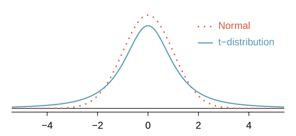
We’ll find it useful to use a new distribution for inference calculations called the $\boldsymbol{t}$ -distribution. A $t$ -distribution, shown as a solid line in Figure 7.1, has a bell shape. However, its tails are thicker than the normal distribution’s, meaning observations are more likely to fall beyond two standard deviations from the mean than under the normal distribution. The extra thick tails of the $t$ -distribution are exactly the correction needed to resolve the problem of using $s$ in place of $\sigma$ in the $SE$ calculation.

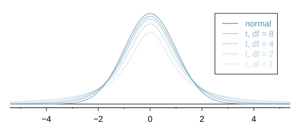
A standard normal distribution and a t-distribution are shown. The t-distribution also has a bell-shape, but it is more sharply peaked than the normal distribution and also has thicker tails than the normal distribution. For example, the is a sizable fraction of the distribution -- perhaps 5% for this particular t-distribution -- that extends below -3 and above positive 3, while the normal distribution is very close to zero when looking below -3 or above positive 3. — **Figure 7.1.** Comparison of a $t$ -distribution and a normal distribution.

The $t$ -distribution is always centered at zero and has a single parameter: degrees of freedom. The degrees of freedom ( $\boldsymbol{df}$ ) describes the precise form of the bell-shaped $t$ -distribution. Several $t$ -distributions are shown in Figure 7.2 in comparison to the normal distribution.

In general, we’ll use a $t$ -distribution with $df = n - 1$ to model the sample mean when the sample size is $n$ . That is, when we have more observations, the degrees of freedom will be larger and the $t$ -distribution will look more like the standard normal distribution; when the degrees of freedom is about 30 or more, the $t$ -distribution is nearly indistinguishable from the normal distribution.

Four t-distributions with degrees of freedom of 1, 2, 4, and 8 are shown along with a normal distribution on the same plot. The larger the degrees of freedom, the more closely the t-distribution aligns with the normal distribution, meaning that the shape of the peak becomes less sharp and the less "thick" the distributions tails appear. — **Figure 7.2.** The larger the degrees of freedom, the more closely the $t$ -distribution resembles the standard normal distribution.

Degrees of freedom ( $\boldsymbol{df}$ )

The degrees of freedom describes the shape of the $t$ -distribution. The larger the degrees of freedom, the more closely the distribution approximates the normal model.

When modeling $\bar{x}$ using the $t$ -distribution, use $df = n - 1$ .

The $t$ -distribution allows us greater flexibility than the normal distribution when analyzing numerical data. In practice, it’s common to use statistical software, such as R, Python, or SAS for these analyses. Alternatively, a graphing calculator or a $\boldsymbol{t}$ -table may be used; the $t$ -table is similar to the normal distribution table, and it may be found in Appendix C.2, which includes usage instructions and examples for those who wish to use this option. No matter the approach you choose, apply your method using the examples below to confirm your working understanding of the $t$ -distribution.

Example 7.2

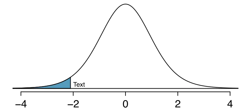
What proportion of the $t$ -distribution with 18 degrees of freedom falls below -2.10?

Just like a normal probability problem, we first draw the picture in Figure 7.3 and shade the area below -2.10. Using statistical software, we can obtain a precise value: 0.0250.

A t-distribution is shown, which is centered at zero. The left tail below -2.1 is shaded, which appears to represent about 2% to 5% of the area under the distribution. — **Figure 7.3.** The $t$ -distribution with 18 degrees of freedom. The area below -2.10 has been shaded.

Example 7.3

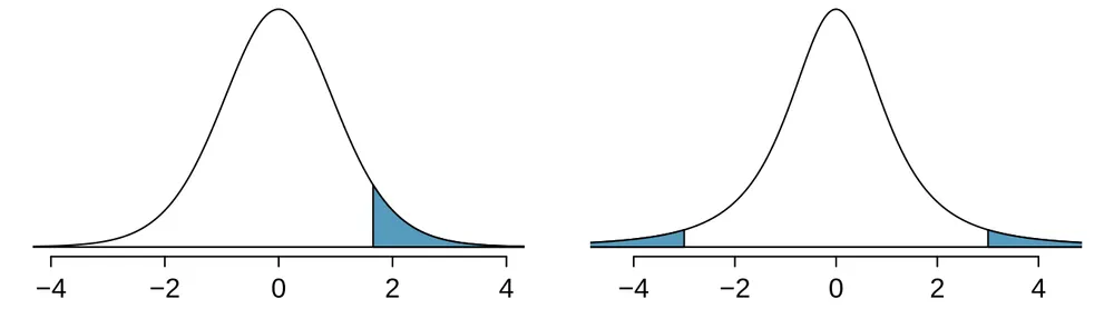
A $t$ -distribution with 20 degrees of freedom is shown in the left panel of Figure 7.4. Estimate the proportion of the distribution falling above 1.65.

With a normal distribution, this would correspond to about 0.05, so we should expect the $t$ -distribution to give us a value in this neighborhood. Using statistical software: 0.0573.

Two t-distributions are shown on two separate plots. The first plot shows a t-distribution with 20 degrees of freedom with the region above positive 1.65 is shaded, which appears to be very roughly 5% of the total distribution area. The second plot shows a t-distribution with 2 degrees of freedom with the region below -3 and above positive 3 shaded. Because the degrees of freedom are so small, the tails are much thicker in this distribution, and its center is also more sharply peaked. Each of these tails appears to represent very roughly 2% to 5% of the area under this distribution. — **Figure 7.4.** Left: The $t$ -distribution with 20 degrees of freedom, with the area above 1.65 shaded. Right: The $t$ -distribution with 2 degrees of freedom, with the area further than 3 units from 0 shaded.

Example 7.4

A $t$ -distribution with 2 degrees of freedom is shown in the right panel of Figure 7.4. Estimate the proportion of the distribution falling more than 3 units from the mean (above or below).

With so few degrees of freedom, the $t$ -distribution will give a more notably different value than the normal distribution. Under a normal distribution, the area would be about 0.003 using the 68-95-99.7 rule. For a $t$ -distribution with $df = 2$ , the area in both tails beyond 3 units totals 0.0955. This area is dramatically different than what we obtain from the normal distribution.

Guided Practice 7.5

What proportion of the $t$ -distribution with 19 degrees of freedom falls above -1.79 units? Use your preferred method for finding tail areas.²

One sample $\boldsymbol{t}$ -confidence intervals

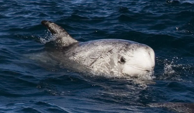
Let’s get our first taste of applying the $t$ -distribution in the context of an example about the mercury content of dolphin muscle. Elevated mercury concentrations are an important problem for both dolphins and other animals, like humans, who occasionally eat them.

A Risso's dolphin is shown surfacing in water. The area forward of its face is mostly white, and then its body is gray and white streaked together. — A Risso’s dolphin.
—————————–
Photo by Mike Baird (www.bairdphotos.com). CC BY 2.0 license.

We will identify a confidence interval for the average mercury content in dolphin muscle using a sample of 19 Risso’s dolphins from the Taiji area in Japan. The data are summarized in Figure 7.6. The minimum and maximum observed values can be used to evaluate whether or not there are clear outliers.

$n$	$\bar{x}$	$s$	minimum	maximum
19	4.4	2.3	1.7	9.2

Figure 7.6. Summary of mercury content in the muscle of 19 Risso’s dolphins from the Taiji area. Measurements are in micrograms of mercury per wet gram of muscle (

\mu

g/wet g).

Example 7.6

Are the independence and normality conditions satisfied for this data set?

The observations are a simple random sample, therefore independence is reasonable. The summary statistics in Figure 7.6 do not suggest any clear outliers, since all observations are within 2.5 standard deviations of the mean. Based on this evidence, the normality condition seems reasonable.

In the normal model, we used $z^{\star}$ and the standard error to determine the width of a confidence interval. We revise the confidence interval formula slightly when using the $t$ -distribution: $\begin{aligned} &\text{point estimate} \ \pm\ t^{\star}_{df} \times SE &&\to &&\bar{x} \ \pm\ t^{\star}_{df} \times \frac{s}{\sqrt{n}} \end{aligned}$

Example 7.7

Using the summary statistics in Figure 7.6, compute the standard error for the average mercury content in the $n = 19$ dolphins.

We plug in $s$ and $n$ into the formula: $SE = s / \sqrt{n} = 2.3 / \sqrt{19} = 0.528$ .

The value $t^{\star}_{df}$ is a cutoff we obtain based on the confidence level and the $t$ -distribution with $df$ degrees of freedom. That cutoff is found in the same way as with a normal distribution: we find $t^{\star}_{df}$ such that the fraction of the $t$ -distribution with $df$ degrees of freedom within a distance $t^{\star}_{df}$ of 0 matches the confidence level of interest.

Example 7.8

When $n = 19$ , what is the appropriate degrees of freedom? Find $t^{\star}_{df}$ for this degrees of freedom and the confidence level of 95%

The degrees of freedom is easy to calculate: $df = n - 1 = 18$ .

Using statistical software, we find the cutoff where the upper tail is equal to 2.5%: $t^{\star}_{18} = 2.10$ . The area below -2.10 will also be equal to 2.5%. That is, 95% of the $t$ -distribution with $df = 18$ lies within 2.10 units of 0.

Example 7.9

Compute and interpret the 95% confidence interval for the average mercury content in Risso’s dolphins.

We can construct the confidence interval as $\begin{aligned} \bar{x} \ \pm\ t^{\star}_{18} \times SE \quad \to \quad 4.4 \ \pm\ 2.10 \times 0.528 \quad \to \quad (3.29, 5.51) \end{aligned}$ We are 95% confident the average mercury content of muscles in Risso’s dolphins is between 3.29 and 5.51 $\mu$ g/wet gram, which is considered extremely high.

Finding a $\boldsymbol{t}$ -confidence interval for the mean

Based on a sample of $n$ independent and nearly normal observations, a confidence interval for the population mean is $\begin{aligned} &\text{point estimate} \ \pm\ t^{\star}_{df} \times SE &&\to &&\bar{x} \ \pm\ t^{\star}_{df} \times \frac{s}{\sqrt{n}} \end{aligned}$ where $\bar{x}$ is the sample mean, $t^{\star}_{df}$ corresponds to the confidence level and degrees of freedom $df$ , and $SE$ is the standard error as estimated by the sample.

Guided Practice 7.10

The FDA’s webpage provides some data on mercury content of fish. Based on a sample of 15 croaker white fish (Pacific), a sample mean and standard deviation were computed as 0.287 and 0.069 ppm (parts per million), respectively. The 15 observations ranged from 0.18 to 0.41 ppm. We will assume these observations are independent. Based on the summary statistics of the data, do you have any objections to the normality condition of the individual observations?³

Example 7.11

Estimate the standard error of $\bar{x} = 0.287$ ppm using the data summaries in Guided Practice 7.10. If we are to use the $t$ -distribution to create a 90% confidence interval for the actual mean of the mercury content, identify the degrees of freedom and $t^{\star}_{df}$ .

The standard error: $SE = \frac{0.069}{\sqrt{15}} = 0.0178$ .

Degrees of freedom: $df = n - 1 = 14$ .

Since the goal is a 90% confidence interval, we choose $t_{14}^{\star}$ so that the two-tail area is 0.1: $t^{\star}_{14} = 1.76$ .

Confidence interval for a single mean

Once you’ve determined a one-mean confidence interval would be helpful for an application, there are four steps to constructing the interval:

Prepare.: Identify $\bar{x}$ , $s$ , $n$ , and determine what confidence level you wish to use.
Check.: Verify the conditions to ensure $\bar{x}$ is nearly normal.
Calculate.: If the conditions hold, compute $SE$ , find $t_{df}^{\star}$ , and construct the interval.
Conclude.: Interpret the confidence interval in the context of the problem.

Guided Practice 7.12

Using the information and results of Guided Practice 7.10 and Example 7.11, compute a 90% confidence interval for the average mercury content of croaker white fish (Pacific).⁴

Guided Practice 7.13

The 90% confidence interval from Guided Practice 7.12 is 0.256 ppm to 0.318 ppm. Can we say that 90% of croaker white fish (Pacific) have mercury levels between 0.256 and 0.318 ppm?⁵

One sample $\boldsymbol{t}$ -tests

the typical US runner getting faster or slower over time? We consider this question in the context of the Cherry Blossom Race, which is a 10-mile race in Washington, DC each spring.

The average time for all runners who finished the Cherry Blossom Race in 2006 was 93.29 minutes (93 minutes and about 17 seconds). We want to determine using data from 100 participants in the 2017 Cherry Blossom Race whether runners in this race are getting faster or slower, versus the other possibility that there has been no change.

Guided Practice 7.14

What are appropriate hypotheses for this context?⁶

Guided Practice 7.15

The data come from a simple random sample of all participants, so the observations are independent. However, should we be worried about the normality condition? See Figure 7.7 for a histogram of the differences and evaluate if we can move forward.⁷

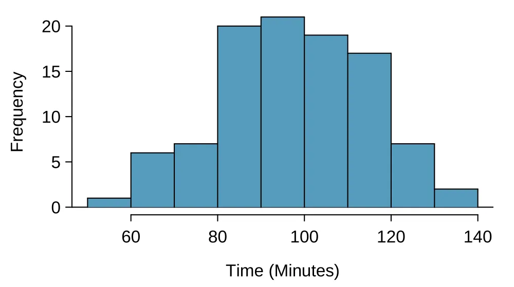
A histogram of "time" for the sample Cherry Blossom Race data is shown. The data are nearly symmetric with a center at about 100 minutes and a standard deviation of roughly 15 to 20 minutes. All times lie between 50 and 140 minutes. — **Figure 7.7.** A histogram of `time` for the sample Cherry Blossom Race data.

When completing a hypothesis test for the one-sample mean, the process is nearly identical to completing a hypothesis test for a single proportion. First, we find the Z-score using the observed value, null value, and standard error; however, we call it a T-score since we use a $t$ -distribution for calculating the tail area. Then we find the p-value using the same ideas we used previously: find the one-tail area under the sampling distribution, and double it.

Example 7.16

With both the independence and normality conditions satisfied, we can proceed with a hypothesis test using the $t$ -distribution. The sample mean and sample standard deviation of the sample of 100 runners from the 2017 Cherry Blossom Race are 97.32 and 16.98 minutes, respectively. Recall that the sample size is 100 and the average run time in 2006 was 93.29 minutes. Find the test statistic and p-value. What is your conclusion?

To find the test statistic (T-score), we first must determine the standard error: $\begin{aligned} SE = 16.98{} / \sqrt{100{}} = 1.70{} \end{aligned}$ Now we can compute the T-score using the sample mean (97.32), null value (93.29), and $SE$ : $\begin{aligned} T = \frac{97.32{} - 93.29{}} {1.70{}} = 2.37{} \end{aligned}$ For $df = 100{} - 1 = 99$ , we can determine using statistical software (or a $t$ -table) that the one-tail area is 0.01, which we double to get the p-value: 0.02.

Because the p-value is smaller than 0.05, we reject the null hypothesis. That is, the data provide strong evidence that the average run time for the Cherry Blossom Run in 2017 is different than the 2006 average. Since the observed value is above the null value and we have rejected the null hypothesis, we would conclude that runners in the race were slower on average in 2017 than in 2006.

Hypothesis testing for a single mean

Once you’ve determined a one-mean hypothesis test is the correct procedure, there are four steps to completing the test:

Prepare.: Identify the parameter of interest, list out hypotheses, identify the significance level, and identify $\bar{x}$ , $s$ , and $n$ .
Check.: Verify conditions to ensure $\bar{x}$ is nearly normal.
Calculate.: If the conditions hold, compute $SE$ , compute the T-score, and identify the p-value.
Conclude.: Evaluate the hypothesis test by comparing the p-value to $\alpha$ , and provide a conclusion in the context of the problem.

Exercises

Exercise 7.1

Identify the critical $t$ . An independent random sample is selected from an approximately normal population with unknown standard deviation. Find the degrees of freedom and the critical $t$ -value (t $^\star$ ) for the given sample size and confidence level.

$n = 6$ , CL = 90%
$n = 21$ , CL = 98%
$n = 29$ , CL = 95%
$n = 12$ , CL = 99%

Exercise 7.2

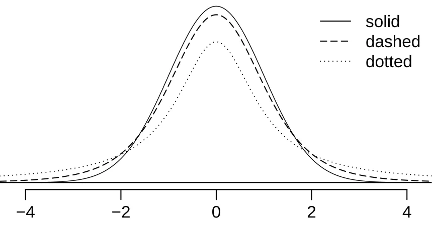
$t$ -distribution. The figure on the right shows three unimodal and symmetric curves: the standard normal (z) distribution, the $t$ -distribution with 5 degrees of freedom, and the $t$ -distribution with 1 degree of freedom. Determine which is which, and explain your reasoning.

Exercise 7.3

Find the p-value, Part I. An independent random sample is selected from an approximately normal population with an unknown standard deviation. Find the p-value for the given sample size and test statistic. Also determine if the null hypothesis would be rejected at $\alpha = 0.05$ .

$n = 11$ , $T = 1.91$
$n = 17$ , $T = -3.45$
$n = 7$ , $T = 0.83$
$n = 28$ , $T = 2.13$

Exercise 7.4

Find the p-value, Part II. An independent random sample is selected from an approximately normal population with an unknown standard deviation. Find the p-value for the given sample size and test statistic. Also determine if the null hypothesis would be rejected at $\alpha = 0.01$ .

$n = 26$ , $T = 2.485$
$n = 18$ , $T = 0.5$

Exercise 7.5

Working backwards, Part I. A 95% confidence interval for a population mean, $\mu$ , is given as (18.985, 21.015). This confidence interval is based on a simple random sample of 36 observations. Calculate the sample mean and standard deviation. Assume that all conditions necessary for inference are satisfied. Use the $t$ -distribution in any calculations.

Exercise 7.6

Working backwards, Part II. A 90% confidence interval for a population mean is (65, 77). The population distribution is approximately normal and the population standard deviation is unknown. This confidence interval is based on a simple random sample of 25 observations. Calculate the sample mean, the margin of error, and the sample standard deviation.

Exercise 7.7

Sleep habits of New Yorkers. New York is known as “the city that never sleeps". A random sample of 25 New Yorkers were asked how much sleep they get per night. Statistical summaries of these data are shown below. The point estimate suggests New Yorkers sleep less than 8 hours a night on average. Is the result statistically significant?

n	$\bar{x}$	s	min	max
25	7.73	0.77	6.17	9.78

Write the hypotheses in symbols and in words.
Check conditions, then calculate the test statistic, $T$ , and the associated degrees of freedom.
Find and interpret the p-value in this context. Drawing a picture may be helpful.
What is the conclusion of the hypothesis test?
If you were to construct a 90% confidence interval that corresponded to this hypothesis test, would you expect 8 hours to be in the interval?

Exercise 7.8

Heights of adults. Researchers studying anthropometry collected body girth measurements and skeletal diameter measurements, as well as age, weight, height and gender, for 507 physically active individuals. The histogram below shows the sample distribution of heights in centimeters. ⁸

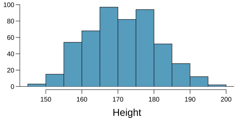
A histogram is shown for "Height" with values ranging from 140 to 200, with a bin width of 5. The distribution is roughly symmetric with a center at about 170. The bin heights, starting with the bin from 145 to 150, are about 3, 17, 55, 70, 100, 85, 95, 50, 30, 15, and 3.

Min	147.2
Q1	163.8
Median	170.3
Mean	171.1
SD	9.4
Q3	177.8
Max	198.1

What is the point estimate for the average height of active individuals? What about the median?
What is the point estimate for the standard deviation of the heights of active individuals? What about the IQR?
Is a person who is 1m 80cm (180 cm) tall considered unusually tall? And is a person who is 1m 55cm (155cm) considered unusually short? Explain your reasoning.
The researchers take another random sample of physically active individuals. Would you expect the mean and the standard deviation of this new sample to be the ones given above? Explain your reasoning.
The sample means obtained are point estimates for the mean height of all active individuals, if the sample of individuals is equivalent to a simple random sample. What measure do we use to quantify the variability of such an estimate? Compute this quantity using the data from the original sample under the condition that the data are a simple random sample.

Exercise 7.9

Find the mean. You are given the following hypotheses: $\begin{aligned} H_0&: \mu = 60 \\ H_A&: \mu \neq 60 \end{aligned}$ We know that the sample standard deviation is 8 and the sample size is 20. For what sample mean would the p-value be equal to 0.05? Assume that all conditions necessary for inference are satisfied.

Exercise 7.10

$t^\star$ vs. $z^\star$ . For a given confidence level, $t^{\star}_{df}$ is larger than $z^{\star}$ . Explain how $t^{*}_{df}$ being slightly larger than $z^{*}$ affects the width of the confidence interval.

Exercise 7.11

Play the piano. Georgianna claims that in a small city renowned for its music school, the average child takes less than 5 years of piano lessons. We have a random sample of 20 children from the city, with a mean of 4.6 years of piano lessons and a standard deviation of 2.2 years.

Evaluate Georgianna’s claim (or that the opposite might be true) using a hypothesis test.
Construct a 95% confidence interval for the number of years students in this city take piano lessons, and interpret it in context of the data.
Do your results from the hypothesis test and the confidence interval agree? Explain your reasoning.

Exercise 7.12

Auto exhaust and lead exposure. Researchers interested in lead exposure due to car exhaust sampled the blood of 52 police officers subjected to constant inhalation of automobile exhaust fumes while working traffic enforcement in a primarily urban environment. The blood samples of these officers had an average lead concentration of 124.32 $\mu$ g/l and a SD of 37.74 $\mu$ g/l; a previous study of individuals from a nearby suburb, with no history of exposure, found an average blood level concentration of 35 $\mu$ g/l.⁹

Write down the hypotheses that would be appropriate for testing if the police officers appear to have been exposed to a different concentration of lead. ·anchor·auto_exhaust_lead_exposure_2_sided_cond· Explicitly state and check all conditions necessary for inference on these data.
Regardless of your answers in part (7.12), test the hypothesis that the downtown police officers have a higher lead exposure than the group in the previous study. Interpret your results in context.

Exercise 7.13

Car insurance savings. A market researcher wants to evaluate car insurance savings at a competing company. Based on past studies he is assuming that the standard deviation of savings is $100. He wants to collect data such that he can get a margin of error of no more than $10 at a 95% confidence level. How large of a sample should he collect?

Exercise 7.14

SAT scores. The standard deviation of SAT scores for students at a particular Ivy League college is 250 points. Two statistics students, Raina and Luke, want to estimate the average SAT score of students at this college as part of a class project. They want their margin of error to be no more than 25 points.

Raina wants to use a 90% confidence interval. How large a sample should she collect?
Luke wants to use a 99% confidence interval. Without calculating the actual sample size, determine whether his sample should be larger or smaller than Raina’s, and explain your reasoning.
Calculate the minimum required sample size for Luke.

an earlier edition of this textbook, we found that Amazon prices were, on average, lower than those of the UCLA Bookstore for UCLA courses in 2010. It’s been several years, and many stores have adapted to the online market, so we wondered, how is the UCLA Bookstore doing today?

We sampled 201 UCLA courses. Of those, 68 required books could be found on Amazon. A portion of the data set from these courses is shown in Figure 7.8, where prices are in US dollars.

	subject	course_number	bookstore	amazon	price_difference
1	American Indian Studies	M10	47.97	47.45	0.52
2	Anthropology	2	14.26	13.55	0.71
3	Arts and Architecture	10	13.50	12.53	0.97
$\vdots$	$\vdots$	$\vdots$	$\vdots$	$\vdots$	$\vdots$
68	Jewish Studies	M10	35.96	32.40	3.56

Figure 7.8. Four cases of the textbooks data set.

Paired observations

Each textbook has two corresponding prices in the data set: one for the UCLA Bookstore and one for Amazon. When two sets of observations have this special correspondence, they are said to be paired.

Paired data

Two sets of observations are paired if each observation in one set has a special correspondence or connection with exactly one observation in the other data set.

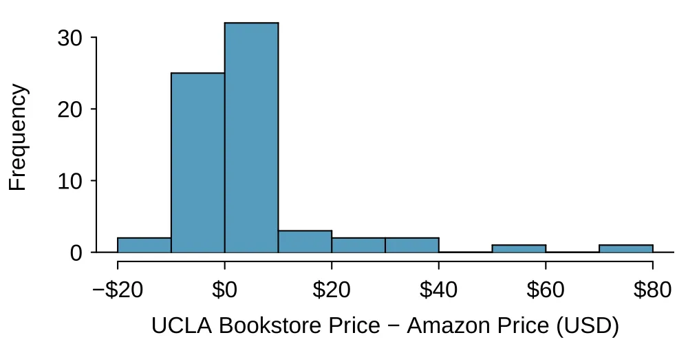
To analyze paired data, it is often useful to look at the difference in outcomes of each pair of observations. In the textbook data, we look at the differences in prices, which is represented as the price_difference variable in the data set. Here the differences are taken as $\begin{aligned} \text{UCLA Bookstore price} - \text{Amazon price} \end{aligned}$ It is important that we always subtract using a consistent order; here Amazon prices are always subtracted from UCLA prices. The first difference shown in Figure 7.8 is computed as $47.97 - 47.45 = 0.52$ . Similarly, the second difference is computed as $14.26 - 13.55 = 0.71$ , and the third is $13.50 - 12.53 = 0.97$ . A histogram of the differences is shown in Figure 7.9. Using differences between paired observations is a common and useful way to analyze paired data.

A histogram is shown for "UCLA bookstore Price minus Amazon Price, in US dollars", where values range from -20 to positive 80. The distribution has a prominent peak at or slightly above 0, with the wide majority of data lying between 20 and positive 20. There are also 4 bins above 20 that have non-zero heights: bin 20 to 30 has a height of 2, bin 30 to 40 has a height of 2, bin 50 to 60 has a height of 1, and bin 70 to 80 has a height of 1. — **Figure 7.9.** Histogram of the difference in price for each book sampled.

Inference for paired data

To analyze a paired data set, we simply analyze the differences. We can use the same $t$ -distribution techniques we applied in Section 7.

$n_{_{\text{\emph{diff}}}}$		$\bar{x}_{_{\text{\emph{diff}}}}$		$s_{_{\text{\emph{diff}}}}$
68		3.58		13.42

Figure 7.10. Summary statistics for the 68 price differences.

Example 7.17

Set up a hypothesis test to determine whether, on average, there is a difference between Amazon’s price for a book and the UCLA bookstore’s price. Also, check the conditions for whether we can move forward with the test using the $t$ -distribution.

We are considering two scenarios: there is no difference or there is some difference in average prices.

$\mu_{\text{\emph{diff}}} = 0$ . There is no difference in the average textbook price.
$\mu_{\text{\emph{diff}}} \neq 0$ . There is a difference in average prices.

Next, we check the independence and normality conditions. The observations are based on a simple random sample, so independence is reasonable. While there are some outliers, $n = 68{}$ and none of the outliers are particularly extreme, so the normality of $\bar{x}$ is satisfied. With these conditions satisfied, we can move forward with the $t$ -distribution.

Example 7.18

Complete the hypothesis test started in Example 7.17.

To compute the test compute the standard error associated with $\bar{x}_{\text{\emph{diff}}}$ using the standard deviation of the differences ( $s_{_{\text{\emph{diff}}}} = 13.42{}$ ) and the number of differences ( $n_{_{\text{\emph{diff}}}} = 68{}$ ): $\begin{aligned} SE_{\bar{x}_{\text{\emph{diff}}}} = \frac{s_{\text{\emph{diff}}}}{\sqrt{n_{\text{\emph{diff}}}}} = \frac{13.42{}}{\sqrt{68{}}} = 1.63{} \end{aligned}$ The test statistic is the T-score of $\bar{x}_{\text{\emph{diff}}}$ under the null condition that the actual mean difference is 0: $\begin{aligned} T = \frac{\bar{x}_{\text{\emph{diff}}} - 0} {SE_{\bar{x}_{\text{\emph{diff}}}}} = \frac{3.58{} - 0}{1.63{}} = 2.20 \end{aligned}$ To visualize the p-value, the sampling distribution of $\bar{x}_{\text{\emph{diff}}}$ is drawn as though $H_0$ is true, and the p-value is represented by the two shaded tails:

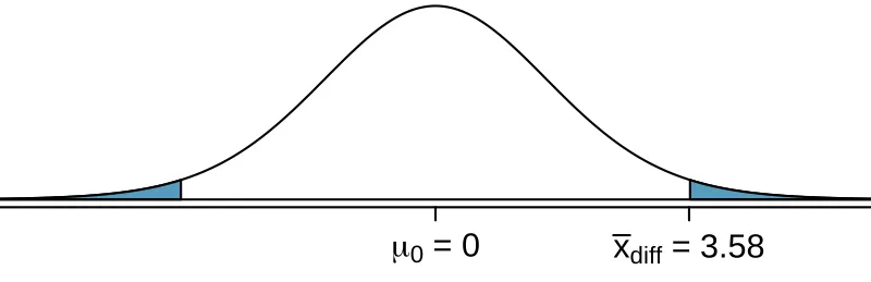
A bell-shaped distribution is shown, with a center of mu-sub-0, which has a value of 0. The area under the distribution above x-bar-sub-diff equals 3.58 is shaded, as is the corresponding tail below -3.58.

The degrees of freedom is $df = 68{} - 1 = 67{}$ . Using statistical software, we find the one-tail area of 0.0156. Doubling this area gives the p-value: 0.0312.

Because the p-value is less than 0.05, we reject the null hypothesis. Amazon prices are, on average, lower than the UCLA Bookstore prices for UCLA courses.

Guided Practice 7.19

Create a 95% confidence interval for the average price difference between books at the UCLA bookstore and books on Amazon.¹⁰

Guided Practice 7.20

We have strong evidence that Amazon is, on average, less expensive. How should this conclusion affect UCLA student buying habits? Should UCLA students always buy their books on Amazon?¹¹

Exercises

Exercise 7.15

Air quality. Air quality measurements were collected in a random sample of 25 country capitals in 2013, and then again in the same cities in 2014. We would like to use these data to compare average air quality between the two years. Should we use a paired or non-paired test? Explain your reasoning.

Exercise 7.16

True / False: paired. Determine if the following statements are true or false. If false, explain.

In a paired analysis we first take the difference of each pair of observations, and then we do inference on these differences.
Two data sets of different sizes cannot be analyzed as paired data.
Consider two sets of data that are paired with each other. Each observation in one data set has a natural correspondence with exactly one observation from the other data set.
Consider two sets of data that are paired with each other. Each observation in one data set is subtracted from the average of the other data set’s observations.

Exercise 7.17

Paired or not? Part I. In each of the following scenarios, determine if the data are paired.

Compare pre- (beginning of semester) and post-test (end of semester) scores of students.
Assess gender-related salary gap by comparing salaries of randomly sampled men and women.
Compare artery thicknesses at the beginning of a study and after 2 years of taking Vitamin E for the same group of patients.
Assess effectiveness of a diet regimen by comparing the before and after weights of subjects.

Exercise 7.18

Paired or not? Part II. In each of the following scenarios, determine if the data are paired.

We would like to know if Intel’s stock and Southwest Airlines’ stock have similar rates of return. To find out, we take a random sample of 50 days, and record Intel’s and Southwest’s stock on those same days.
We randomly sample 50 items from Target stores and note the price for each. Then we visit Walmart and collect the price for each of those same 50 items.
A school board would like to determine whether there is a difference in average SAT scores for students at one high school versus another high school in the district. To check, they take a simple random sample of 100 students from each high school.

Exercise 7.19

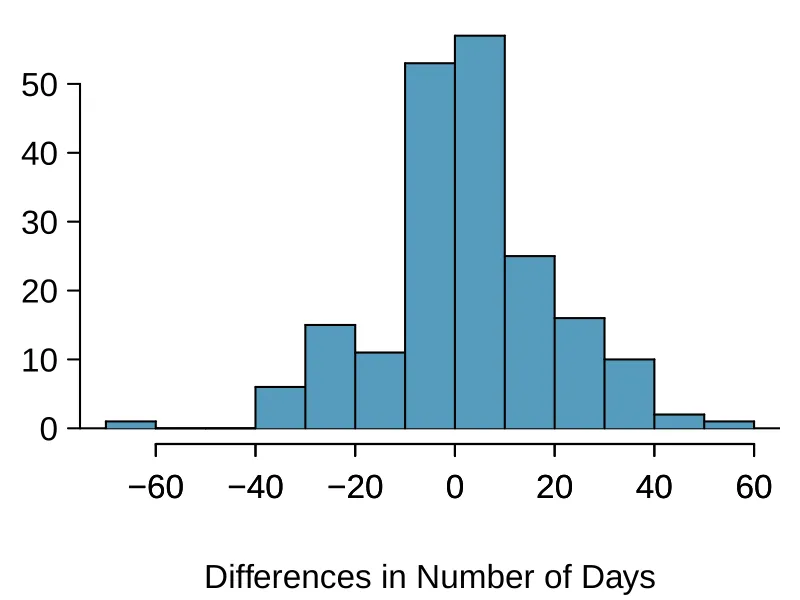
Global warming, Part I. Let’s consider a limited set of climate data, examining temperature differences in 1948 vs 2018. We sampled 197 locations from the National Oceanic and Atmospheric Administration’s (NOAA) historical data, where the data was available for both years of interest. We want to know: were there more days with temperatures exceeding 90F in 2018 or in 1948?¹² The difference in number of days exceeding 90F (number of days in 2018 - number of days in 1948) was calculated for each of the 197 locations. The average of these differences was 2.9 days with a standard deviation of 17.2 days. We are interested in determining whether these data provide strong evidence that there were more days in 2018 that exceeded 90F from NOAA’s weather stations.

Is there a relationship between the observations collected in 1948 and 2018? Or are the observations in the two groups independent? Explain.
Write hypotheses for this research in symbols and in words.
Check the conditions required to complete this test. A histogram of the differences is given to the right.
Calculate the test statistic and find the p-value.
Use $\alpha = 0.05$ to evaluate the test, and interpret your conclusion in context.
What type of error might we have made? Explain in context what the error means.
Based on the results of this hypothesis test, would you expect a confidence interval for the average difference between the number of days exceeding 90F from 1948 and 2018 to include 0? Explain your reasoning.

A histogram is shown for "Differences in Number of Days", which has bins between -70 and 60, where the bin width is 10. There is a prominent peak around zero, where much of the data lies between -40 and positive 40. The non-zero bins beyond this range are -70 to -60 has a bin height of 1, the 40 to 50 bin has a bin height of 2, and the 50 to 60 bin has a bin height of 1.

Exercise 7.20

High School and Beyond, Part I. The National Center of Education Statistics conducted a survey of high school seniors, collecting test data on reading, writing, and several other subjects. Here we examine a simple random sample of 200 students from this survey. Side-by-side box plots of reading and writing scores as well as a histogram of the differences in scores are shown below.

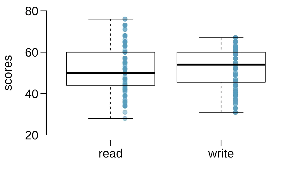
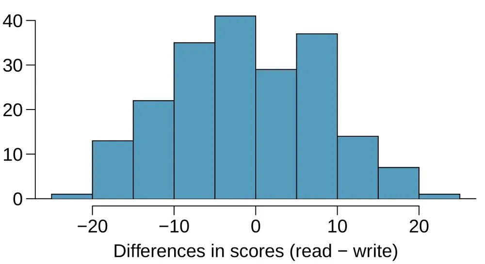
Is there a clear difference in the average reading and writing scores?
Are the reading and writing scores of each student independent of each other?
Create hypotheses appropriate for the following research question: is there an evident difference in the average scores of students in the reading and writing exam?
Check the conditions required to complete this test.
The average observed difference in scores is $\bar{x}_{read-write} = -0.545$ , and the standard deviation of the differences is 8.887 points. Do these data provide convincing evidence of a difference between the average scores on the two exams?
What type of error might we have made? Explain what the error means in the context of the application.
Based on the results of this hypothesis test, would you expect a confidence interval for the average difference between the reading and writing scores to include 0? Explain your reasoning.

Exercise 7.21

Global warming, Part II. We considered the change in the number of days exceeding 90F from 1948 and 2018 at 197 randomly sampled locations from the NOAA database in Exercise 7.19. The mean and standard deviation of the reported differences are 2.9 days and 17.2 days.

Calculate a 90% confidence interval for the average difference between number of days exceeding 90F between 1948 and 2018. We’ve already checked the conditions for you.
Interpret the interval in context.
Does the confidence interval provide convincing evidence that there were more days exceeding 90F in 2018 than in 1948 at NOAA stations? Explain.

Exercise 7.22

High school and beyond, Part II. We considered the differences between the reading and writing scores of a random sample of 200 students who took the High School and Beyond Survey in Exercise 7.20. The mean and standard deviation of the differences are $\bar{x}_{read-write} = -0.545$ and 8.887 points.

Calculate a 95% confidence interval for the average difference between the reading and writing scores of all students.
Interpret this interval in context.
Does the confidence interval provide convincing evidence that there is a real difference in the average scores? Explain.

Notes

More nuanced guidelines would consider further relaxing the particularly extreme outlier check when the sample size is very large. However, we’ll leave further discussion here to a future course. ↩
We want to find the shaded area above -1.79 (we leave the picture to you). The lower tail area has an area of 0.0447, so the upper area would have an area of $1 - 0.0447 = 0.9553$ . ↩
The sample size is under 30, so we check for obvious outliers: since all observations are within 2 standard deviations of the mean, there are no such clear outliers. ↩
$\bar{x} \ \pm\ t^{\star}_{14} \times SE \ \to\ 0.287 \ \pm\ 1.76 \times 0.0178 \ \to\ (0.256, 0.318)$ . We are 90% confident that the average mercury content of croaker white fish (Pacific) is between 0.256 and 0.318 ppm. ↩
No, a confidence interval only provides a range of plausible values for a population parameter, in this case the population mean. It does not describe what we might observe for individual observations. ↩
$H_0$ : The average 10-mile run time was the same for 2006 and 2017. $\mu = 93.29{}$ minutes. $H_A$ : The average 10-mile run time for 2017 was different than that of 2006. $\mu \neq 93.29{}$ minutes. ↩
With a sample of 100, we should only be concerned if there is are particularly extreme outliers. The histogram of the data doesn’t show any outliers of concern (and arguably, no outliers at all). ↩
Heinz, G. et al. Exploring relationships in body dimensions. Journal of Statistics Education. 2003. ↩
Mortada, WI et al. Study of lead exposure from automobile exhaust as a risk for nephrotoxicity among traffic policemen. American journal of nephrology. 2000. ↩
Conditions have already verified and the standard error computed in Example 7.17. To find the interval, identify $t^{\star}_{67{}}$ using statistical software or the $t$ -table ( $t^{\star}_{67{}} = 2.00$ ), and plug it, the point estimate, and the standard error into the confidence interval formula: $\begin{aligned} \text{point estimate} \ \pm\ z^{\star} \times SE \quad\to\quad 3.58{} \ \pm\ 2.00 \times 1.63{} \quad\to\quad (0.32, 6.84) \end{aligned}$ We are 95% confident that Amazon is, on average, between $0.32 and $6.84 less expensive than the UCLA Bookstore for UCLA course books. ↩
The average price difference is only mildly useful for this question. Examine the distribution shown in Figure 7.9. There are certainly a handful of cases where Amazon prices are far below the UCLA Bookstore’s, which suggests it is worth checking Amazon (and probably other online sites) before purchasing. However, in many cases the Amazon price is above what the UCLA Bookstore charges, and most of the time the price isn’t that different. Ultimately, if getting a book immediately from the bookstore is notably more convenient, e.g. to get started on reading or homework, it’s likely a good idea to go with the UCLA Bookstore unless the price difference on a specific book happens to be quite large.

For reference, this is a very different result from what we (the authors) had seen in a similar data set from 2010. At that time, Amazon prices were almost uniformly lower than those of the UCLA Bookstore’s and by a large margin, making the case to use Amazon over the UCLA Bookstore quite compelling at that time. Now we frequently check multiple websites to find the best price. ↩
NOAA, www.ncdc.noaa.gov/cdo-web/datasets, April 24, 2019. ↩

Build status · Flash Infinity AI™ is a trademark of AI-Flash Inc.. WorldClass is not affiliated with, approved or accredited by any exam board, curriculum provider or university unless a page says so.

Paired data

The sampling distribution of xˉ\boldsymbol{\bar{x}}

Evaluating the two conditions required for modeling xˉ\boldsymbol{\bar{x}}

Introducing the t\boldsymbol{t}-distribution

One sample t\boldsymbol{t}-confidence intervals

One sample t\boldsymbol{t}-tests

Exercises

Paired observations

Inference for paired data

Exercises

Notes

The sampling distribution of $\boldsymbol{\bar{x}}$

Evaluating the two conditions required for modeling $\boldsymbol{\bar{x}}$

Introducing the $\boldsymbol{t}$ -distribution

One sample $\boldsymbol{t}$ -confidence intervals

One sample $\boldsymbol{t}$ -tests