In this section, we identify criteria for determining which outliers are important and influential. Outliers in regression are observations that fall far from the cloud of points. These points are especially important because they can have a strong influence on the least squares line.
Example 8.17
There are six plots shown in Figure 8.18 along with the least squares line and residual plots. For each scatterplot and residual plot pair, identify the outliers and note how they influence the least squares line. Recall that an outlier is any point that doesn’t appear to belong with the vast majority of the other points.
There is one outlier far from the other points, though it only appears to slightly influence the line.
There is one outlier on the right, though it is quite close to the least squares line, which suggests it wasn’t very influential.
There is one point far away from the cloud, and this outlier appears to pull the least squares line up on the right; examine how the line around the primary cloud doesn’t appear to fit very well.
There is a primary cloud and then a small secondary cloud of four outliers. The secondary cloud appears to be influencing the line somewhat strongly, making the least square line fit poorly almost everywhere. There might be an interesting explanation for the dual clouds, which is something that could be investigated.
There is no obvious trend in the main cloud of points and the outlier on the right appears to largely control the slope of the least squares line.
There is one outlier far from the cloud. However, it falls quite close to the least squares line and does not appear to be very influential.
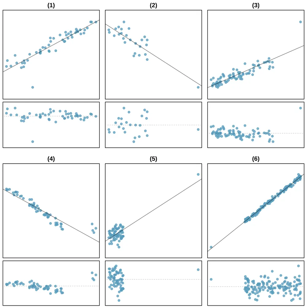
Examine the residual plots in Figure 8.18. You will probably find that there is some trend in the main clouds of (3) and (4). In these cases, the outliers influenced the slope of the least squares lines. In (5), data with no clear trend were assigned a line with a large trend simply due to one outlier (!).
Leverage
Points that fall horizontally away from the center of the cloud tend to pull harder on the line, so we call them points with high leverage.
Points that fall horizontally far from the line are points of high leverage; these points can strongly influence the slope of the least squares line. If one of these high leverage points does appear to actually invoke its influence on the slope of the line – as in cases (3), (4), and (5) of Example 8.17 – then we call it an influential point. Usually we can say a point is influential if, had we fitted the line without it, the influential point would have been unusually far from the least squares line.
It is tempting to remove outliers. Don’t do this without a very good reason. Models that ignore exceptional (and interesting) cases often perform poorly. For instance, if a financial firm ignored the largest market swings – the “outliers” – they would soon go bankrupt by making poorly thought-out investments.
Exercises
Exercise 8.27
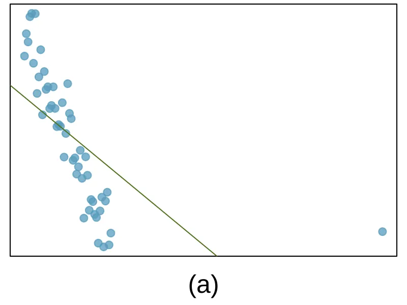
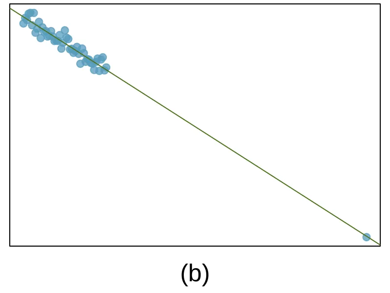
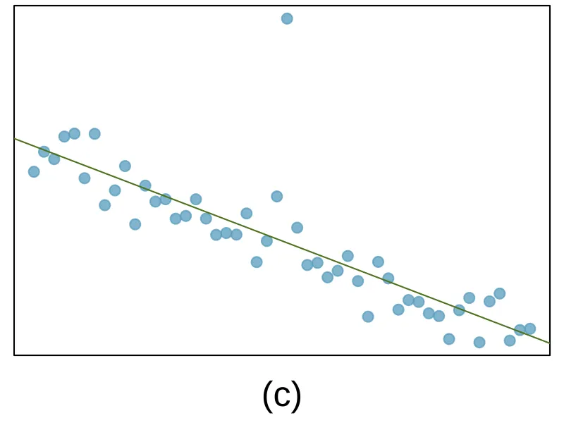
Outliers, Part I. Identify the outliers in the scatterplots shown below, and determine what type of outliers they are. Explain your reasoning.
Exercise 8.28
Outliers, Part II. Identify the outliers in the scatterplots shown below and determine what type of outliers they are. Explain your reasoning.
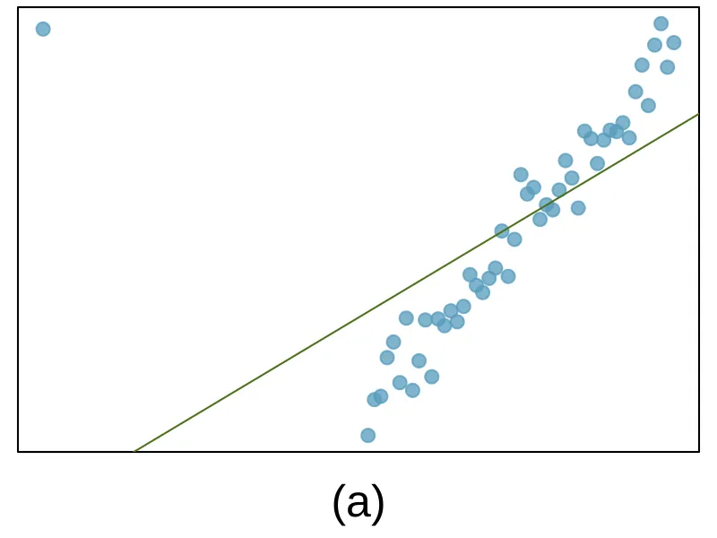
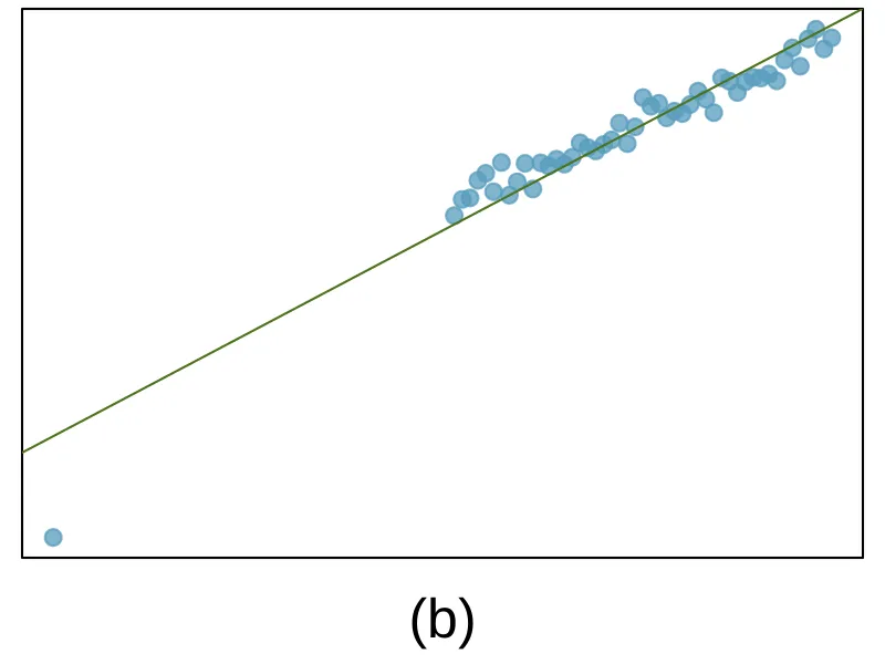
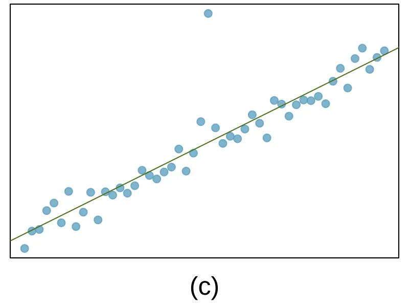
Exercise 8.29
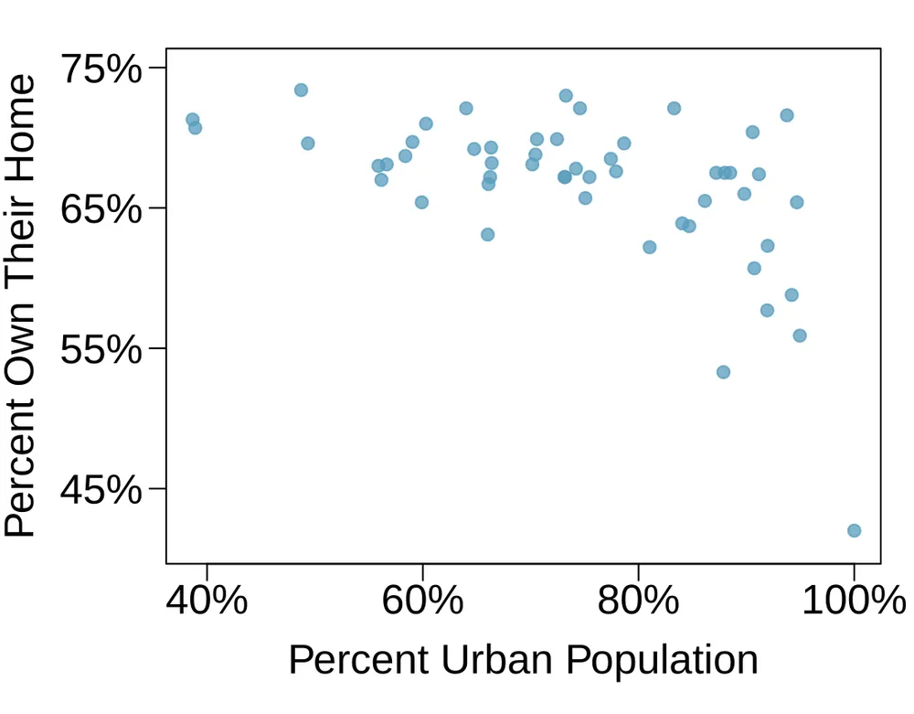
Urban homeowners, Part I. The scatterplot below shows the percent of families who own their home vs. the percent of the population living in urban areas. 1 There are 52 observations, each corresponding to a state in the US. Puerto Rico and District of Columbia are also included.
Describe the relationship between the percent of families who own their home and the percent of the population living in urban areas.
The outlier at the bottom right corner is District of Columbia, where 100% of the population is considered urban. What type of an outlier is this observation?
Exercise 8.30
Crawling babies, Part II. Exercise 8.12 introduces data on the average monthly temperature during the month babies first try to crawl (about 6 months after birth) and the average first crawling age for babies born in a given month. A scatterplot of these two variables reveals a potential outlying month when the average temperature is about 53^F and average crawling age is about 28.5 weeks. Does this point have high leverage? Is it an influential point?
Notes
United States Census Bureau, 2010 Census Urban and Rural Classification and Urban Area Criteria and Housing Characteristics: 2010. ↩