regression methods using the model generally depend on the following four conditions:
the residuals of the model are nearly normal (less important for larger data sets),
the variability of the residuals is nearly constant,
the residuals are independent, and
each variable is linearly related to the outcome.
Diagnostic plots
Diagnostic plots can be used to check each of these conditions. We will consider the model from the Lending Club loans data, and check whether there are any notable concerns:
- Check for outliers.
-
In theory, the distribution of the residuals should be nearly normal; in practice, normality can be relaxed for most applications. Instead, we examine a histogram of the residuals to check if there are any outliers: Figure 9.8 is a histogram of these outliers. Since this is a very large data set, only particularly extreme observations would be a concern in this particular case. There are no extreme observations that might cause a concern.
If we intended to construct what are called prediction intervals for future observations, we would be more strict and require the residuals to be nearly normal. Prediction intervals are further discussed in an online extra on the OpenIntro website:
www.openintro.org/d?id=stat_extra_linear_regression_supp
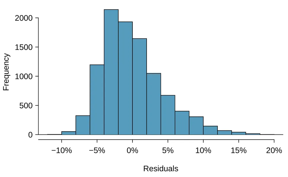
Figure 9.8. A histogram of the residuals. - Absolute values of residuals against fitted values.
-
A plot of the absolute value of the residuals against their corresponding fitted values () is shown in Figure 9.9. This plot is helpful to check the condition that the variance of the residuals is approximately constant, and a smoothed line has been added to represent the approximate trend in this plot. There is more evident variability for fitted values that are larger, which we’ll discuss further.
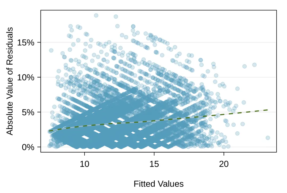
Figure 9.9. Comparing the absolute value of the residuals against the fitted values () is helpful in identifying deviations from the constant variance assumption. - Residuals in order of their data collection.
-
This type of plot can be helpful when observations were collected in a sequence. Such a plot is helpful in identifying any connection between cases that are close to one another. The loans in this data set were issued over a 3 month period, and the month the loan was issued was not found to be important, suggesting this is not a concern for this data set. In cases where a data set does show some pattern for this check, time series methods may be useful.
- Residuals against each predictor variable.
-
We consider a plot of the residuals against each of the predictors in Figure 9.10. For those instances where there are only 2-3 groups, box plots are shown. For the numerical outcomes, a smoothed line has been fit to the data to make it easier to review. Ultimately, we are looking for any notable change in variability between groups or pattern in the data.
Here are the things of importance from these plots:
There is some minor differences in variability between the verified income groups.
There is a very clear pattern for the debt-to-income variable. What also stands out is that this variable is very strongly right skewed: there are few observations with very high debt-to-income ratios.
The downward curve on the right side of the credit utilization and credit check plots suggests some minor misfitting for those larger values.
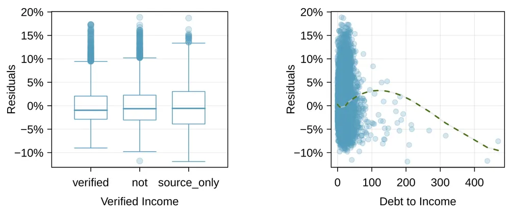
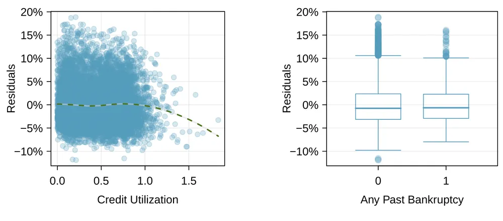
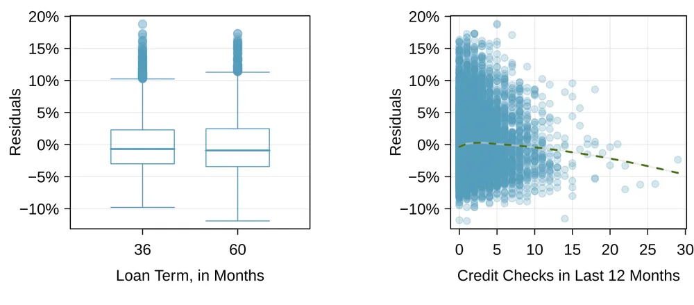
Figure 9.10. Diagnostic plots for residuals against each of the predictors. For the box plots, we’re looking for notable differences in variability. For numerical predictors, we also check for trends or other structure in the data.
Having reviewed the diagnostic plots, there are two options. The first option is to, if we’re not concerned about the issues observed, use this as the final model; if going this route, it is important to still note any abnormalities observed in the diagnostics. The second option is to try to improve the model, which is what we’ll try to do with this particular model fit.
Options for improving the model fit
There are several options for improvement of a model, including transforming variables, seeking out additional variables to fill model gaps, or using more advanced methods that would account for challenges around inconsistent variability or nonlinear relationships between predictors and the outcome.
The main concern for the initial model is that there is a notable nonlinear relationship between the debt-to-income variable observed in Figure 9.10. To resolve this issue, we’re going to consider a couple strategies for adjusting the relationship between the predictor variable and the outcome.
Let’s start by taking a look at a histogram of debt_to_income in Figure 9.11. The variable is extremely skewed, and upper values will have a lot of leverage on the fit. Below are several options:
log transformation (),
square root transformation (),
inverse transformation (),
truncation (cap the max value possible)
If we inspected the data more closely, we’d observe some instances where the variable takes a value of 0, and since and are undefined when , we’ll exclude these transformations from further consideration.1 A square root transformation is valid for all values the variable takes, and truncating some of the larger observations is also a valid approach. We’ll consider both of these approaches.
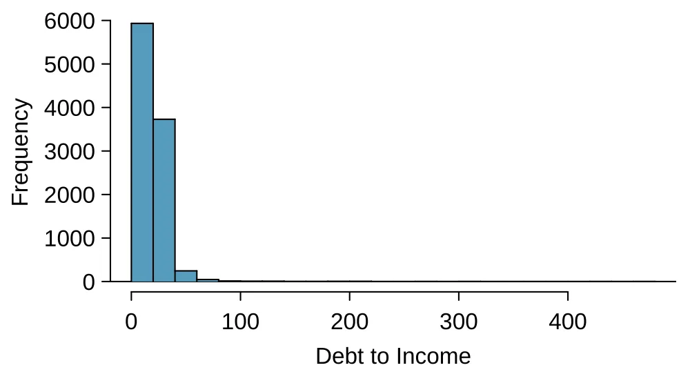
debt_to_income, where extreme skew is evident.To try transforming the variable, we make two new variables representing the transformed versions:
- Square root.
-
We create a new variable,
sqrt_debt_to_income, where all the values are simply the square roots of the values indebt_to_income, and then refit the model as before. The result is shown in the left panel of Figure 9.12. The square root pulled in the higher values a bit, but the fit still doesn’t look great since the smoothed line is still wavy. - Truncate at 50.
-
We create a new variable,
debt_to_income_50, where any values indebt_to_incomethat are greater than 50 are shrunk to exactly 50. Refitting the model once more, the diagnostic plot for this new variable is shown in the right panel of Figure 9.12. Here the fit looks much more reasonable, so this appears to be a reasonable approach.
The downside of using transformations is that it reduces the ease of interpreting the results. Fortunately, since the truncation transformation only affects a relatively small number of cases, the interpretation isn’t dramatically impacted.
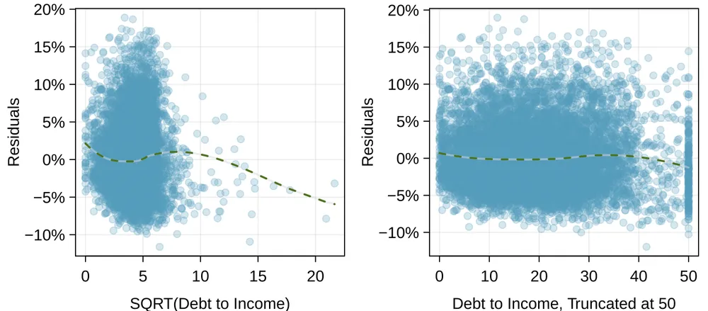
debt_to_income, where extreme skew is evident.As a next step, we’d evaluate the new model using the truncated version of debt_to_income, we would complete all the same procedures as before. The other two issues noted while inspecting diagnostics in Section 9.3.1 are still present in the updated model. If we choose to report this model, we would want to also discuss these shortcomings to be transparent in our work. Depending on what the model will be used for, we could either try to bring those under control, or we could stop since those issues aren’t severe. Had the non-constant variance been a little more dramatic, it would be a higher priority. Ultimately we decided that the model was reasonable, and we report its final form here: A sharp eye would notice that the coefficient for debt_to_income_50 is more than twice as large as what the coefficient had been for the debt_to_income variable in the earlier model. This suggests those larger values not only were points with high leverage, but they were influential points that were dramatically impacting the coefficient.
“All models are wrong, but some are useful” -George E.P. Box
The truth is that no model is perfect. However, even imperfect models can be useful. Reporting a flawed model can be reasonable so long as we are clear and report the model’s shortcomings.
Don’t report results when conditions are grossly violated. While there is a little leeway in model conditions, don’t go too far. If model conditions are very clearly violated, consider a new model, even if it means learning more statistical methods or hiring someone who can help. To help you get started, we’ve developed a couple additional sections that you may find on OpenIntro’s website. These sections provide a light introduction to what are called interaction terms
and to fitting nonlinear curves to data, respectively:
www.openintro.org/d?file=stat_extra_interaction_effects
www.openintro.org/d?file=stat_extra_nonlinear_relationships
Exercises
Exercise 9.13
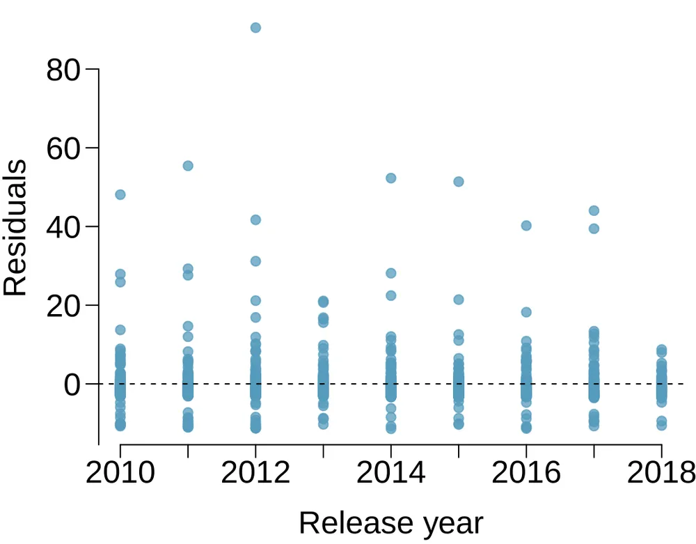
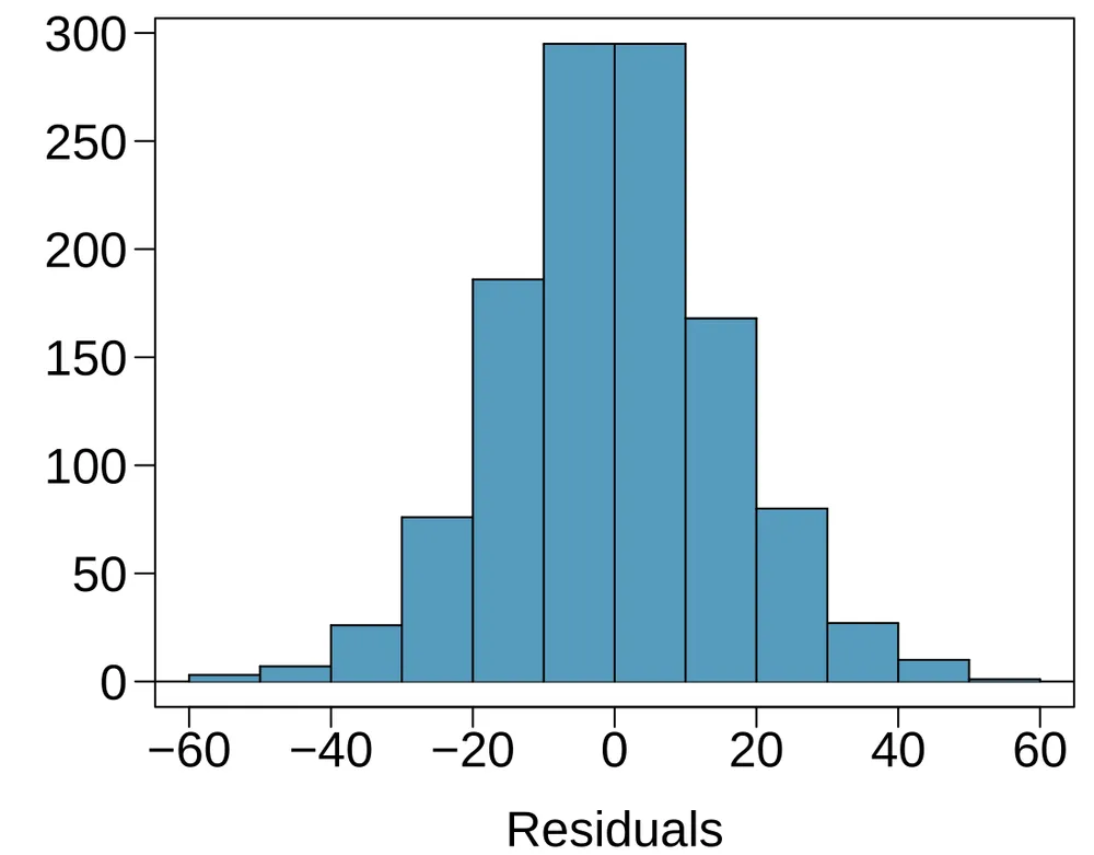
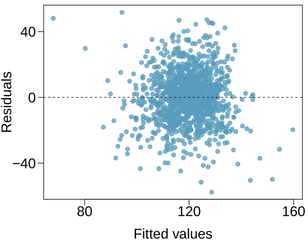
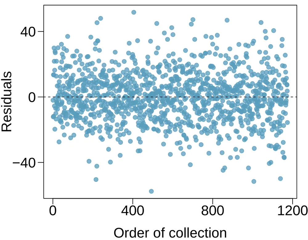
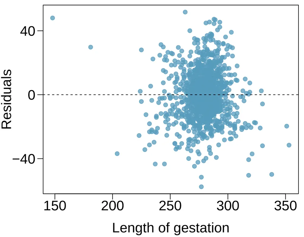
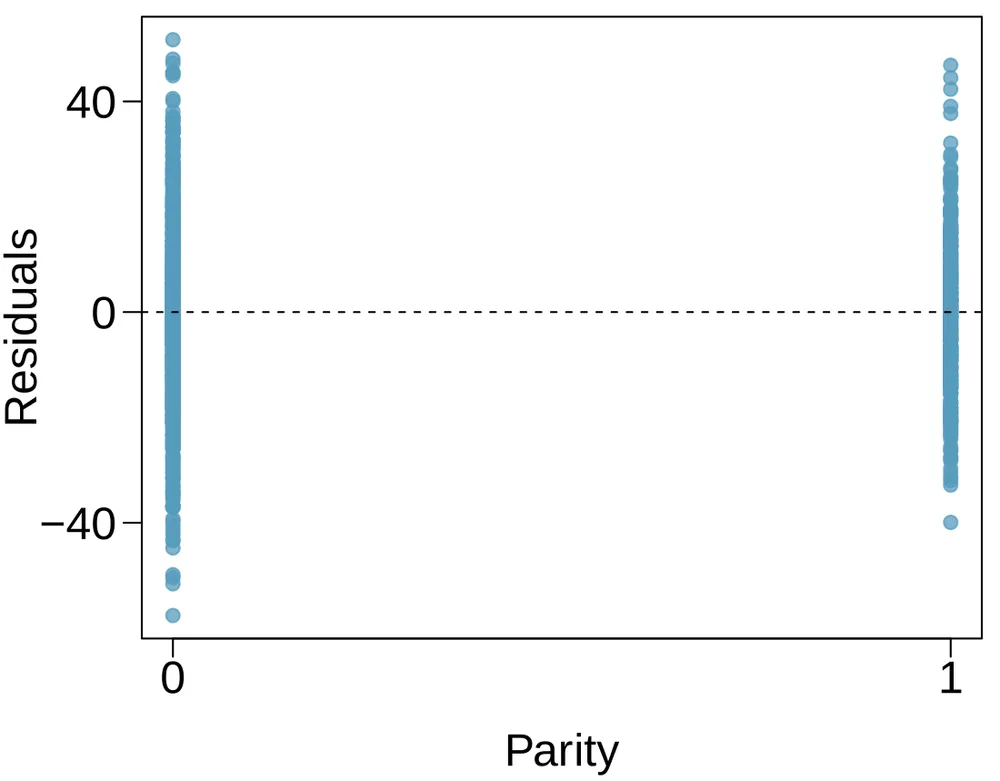
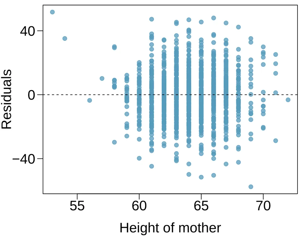
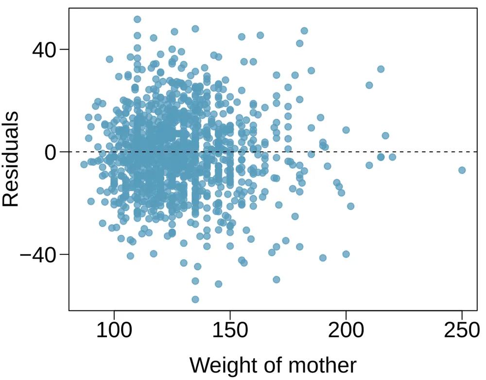
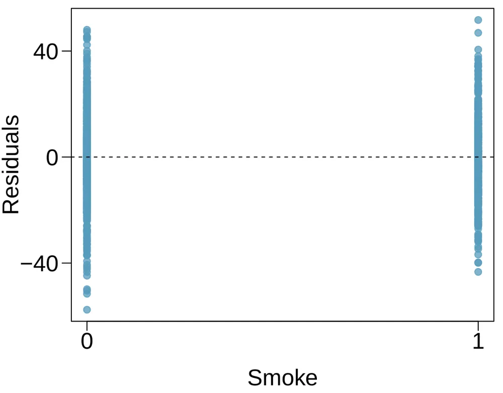
Baby weights, Part VI. Exercise 9.3 presents a regression model for predicting the average birth weight of babies based on length of gestation, parity, height, weight, and smoking status of the mother. Determine if the model assumptions are met using the plots below. If not, describe how to proceed with the analysis.
Exercise 9.14
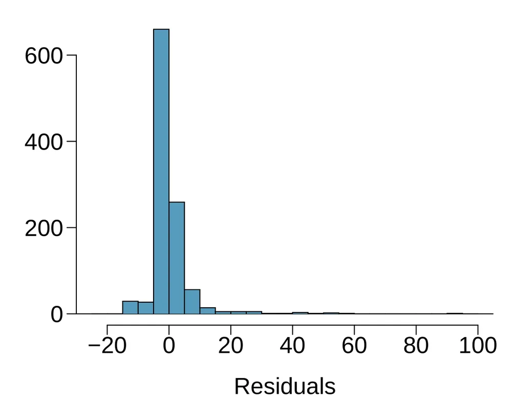
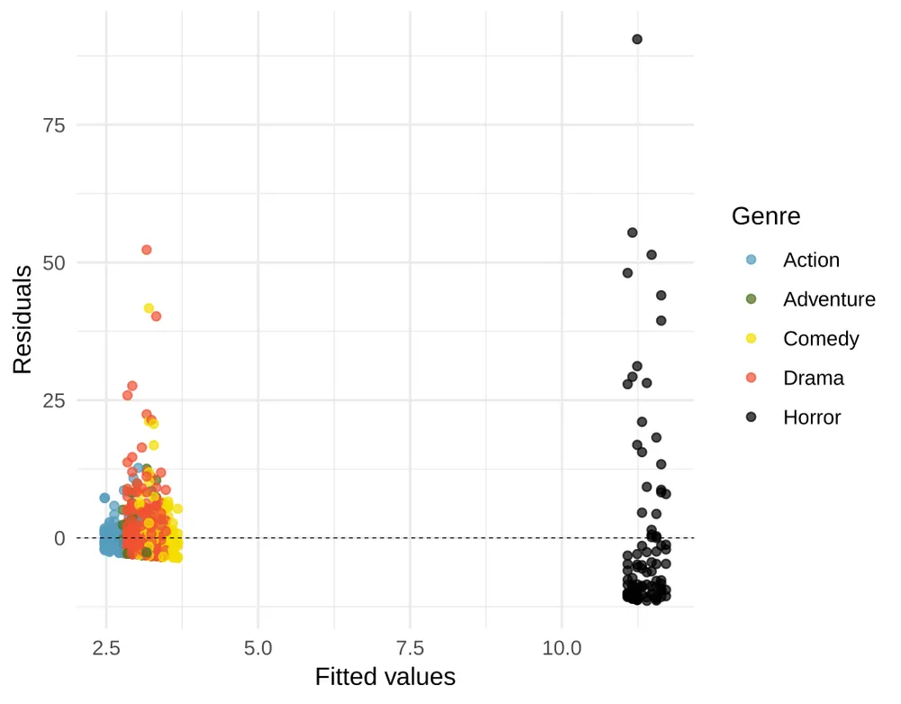
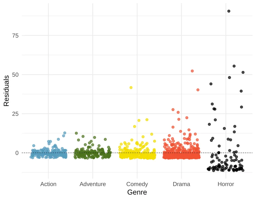
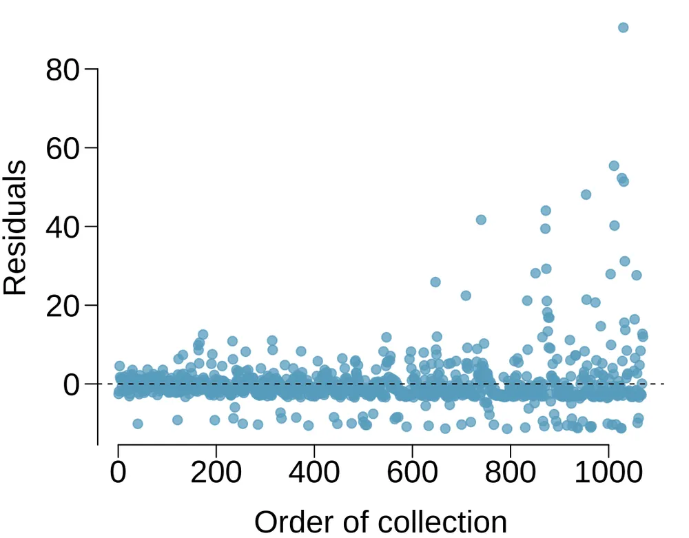
Movie returns, Part I. A FiveThirtyEight.com article reports that “Horror movies get nowhere near as much draw at the box office as the big-time summer blockbusters or action/adventure movies ... but there’s a huge incentive for studios to continue pushing them out. The return-on-investment potential for horror movies is absurd." To investigate how the return-on-investment compares between genres and how this relationship has changed over time, an introductory statistics student fit a model predicting the ratio of gross revenue of movies from genre and release year for 1,070 movies released between 2000 and 2018. Using the plots given below, determine if this regression model is appropriate for these data.2