Motivating Questions
- Given a function of two independent variables and how are the second-order partial derivatives of defined?
- What do the second-order partial derivatives and of a function tell us about the function's behavior?
Recall that for a single-variable function the second derivative of is defined to be the derivative of the first derivative. That is, which can be stated in terms of the limit definition of the derivative by writing
In what follows, we begin exploring the four different second-order partial derivatives of a function of two variables and seek to understand what these various derivatives tell us about the function's behavior.
Preview Activity
Once again, let's consider the function defined by that measures a projectile's range as a function of its initial speed and launch angle The graph of this function, including traces with and is shown in Figure .
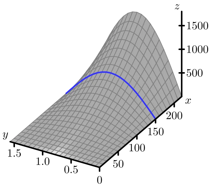
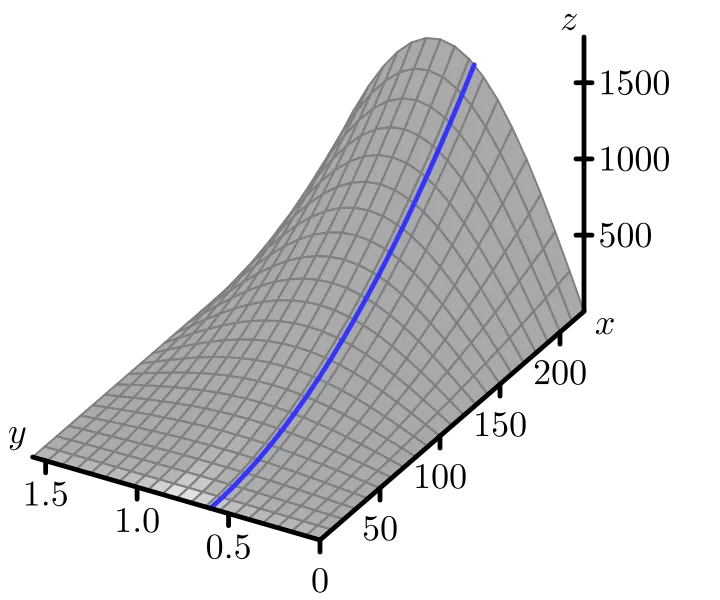
a. Compute the partial derivative Notice that itself is a new function of and so we may now compute the partial derivatives of Find the partial derivative and show that
b. Figure shows the trace of with with three tangent lines included. Explain how your result from part (a) of this preview activity is reflected in this figure.
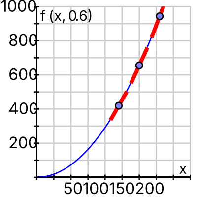
c. Determine the partial derivative and then find the partial derivative Evaluate
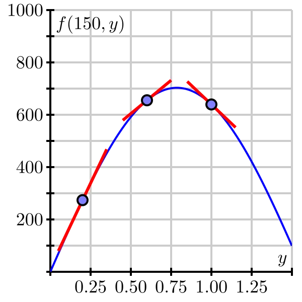
d. Figure shows the trace and includes three tangent lines. Explain how the value of is reflected in this figure.
e. Because and are each functions of both and they each have two partial derivatives. Not only can we compute but also likewise, in addition to but also For the range function use your earlier computations of and to now determine and Write one sentence to explain how you calculated these “mixed” partial derivatives.
A function of two independent variables and has two first order partial derivatives, and As we saw in Preview Activity , each of these first-order partial derivatives has two partial derivatives, giving a total of four second-order partial derivatives:
The first two are called unmixed second-order partial derivatives while the last two are called the mixed second-order partial derivatives.
One aspect of this notation can be a little confusing. The notation
means that we first differentiate with respect to and then with respect to this can be expressed in the alternate notation However, to find the second partial derivative
we first differentiate with respect to and then This means that
Be sure to note carefully the difference between Leibniz notation and subscript notation and the order in which and appear in each. In addition, remember that anytime we compute a partial derivative, we hold constant the variable(s) other than the one we are differentiating with respect to.
Activity
Find all second order partial derivatives of the following functions. For each partial derivative you calculate, state explicitly which variable is being held constant.
- How many second order partial derivatives does the function defined by have? Find and (you do not need to find the other second order partial derivatives).
In Preview Activity and Activity , you may have noticed that the mixed second-order partial derivatives are equal. This observation holds generally and is known as Clairaut's Theorem.
Clairaut's Theorem
Let be a function of several variables for which the partial derivatives and are continuous near the point Then
Interpreting the Second-Order Partial Derivatives
Recall from single variable calculus that the second derivative measures the instantaneous rate of change of the derivative. This observation is the key to understanding the meaning of the second-order partial derivatives.
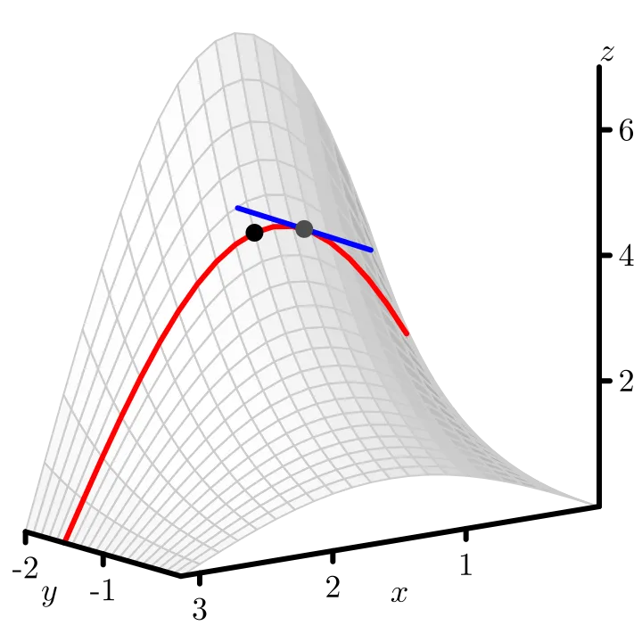
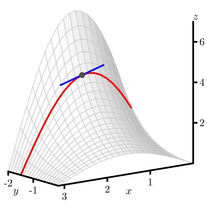
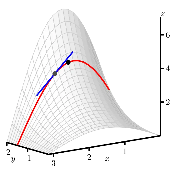
Furthermore, we remember that the second derivative of a function at a point provides us with information about the concavity of the function at that point. Since the unmixed second-order partial derivative requires us to hold constant and differentiate twice with respect to we may simply view as the second derivative of a trace of where is fixed. As such, will measure the concavity of this trace.
Consider, for example, Figure shows the graph of this function along with the trace given by Also shown are three tangent lines to this trace, with increasing -values from left to right among the three plots in Figure .
That the slope of the tangent line is decreasing as increases is reflected, as it is in one-variable calculus, in the fact that the trace is concave down. Indeed, we see that and so since for all values of including
In the following activity, we further explore what second-order partial derivatives tell us about the geometric behavior of a surface.
Activity
We continue to consider the function defined by
a. In Figure , we see the trace of that has held constant with We also see three different lines that are tangent to the trace of in the direction at values of that are increasing from left to right in the figure. Write a couple of sentences that describe whether the slope of the tangent lines to this curve increase or decrease as increases, and, after computing explain how this observation is related to the value of Be sure to address the notion of concavity in your response.(You need to be careful about the directions in which and are increasing.)
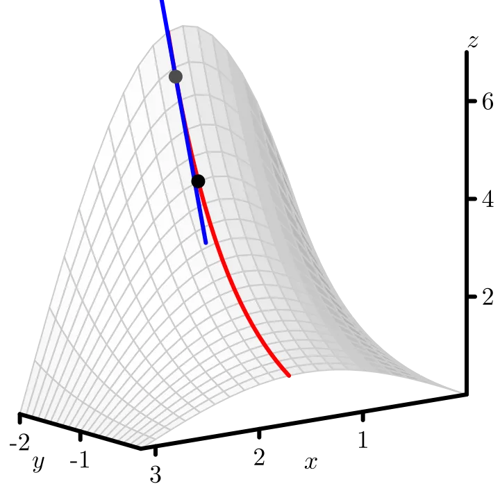
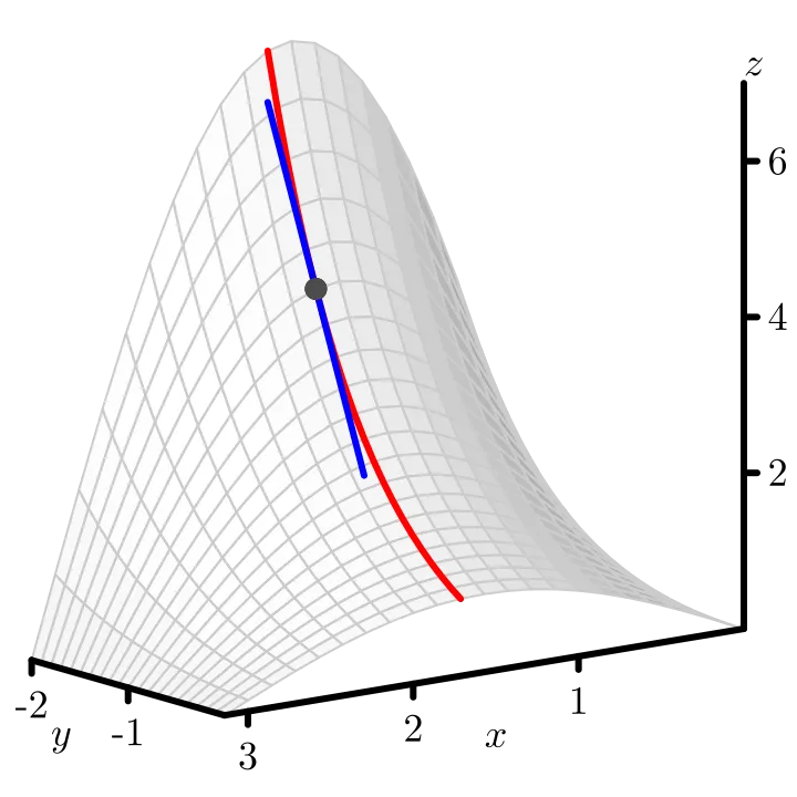
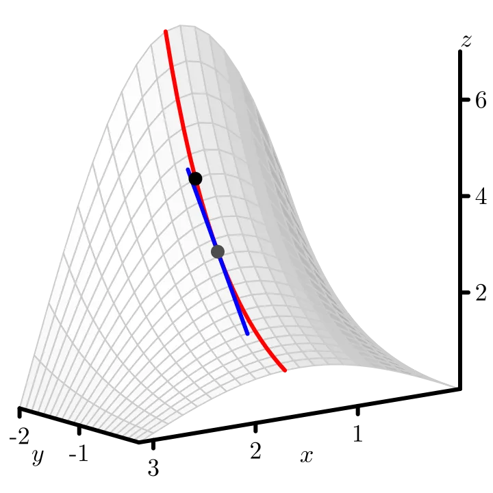
b. In Figure , we start to think about the mixed partial derivative, Here, we first hold constant to generate the first-order partial derivative and then we hold constant to compute This leads to first thinking about a trace with being constant, followed by slopes of tangent lines in the -direction that slide along the original trace. You might think of sliding your pencil down the trace with constant in a way that its slope indicates in order to further animate the three snapshots shown in the figure.
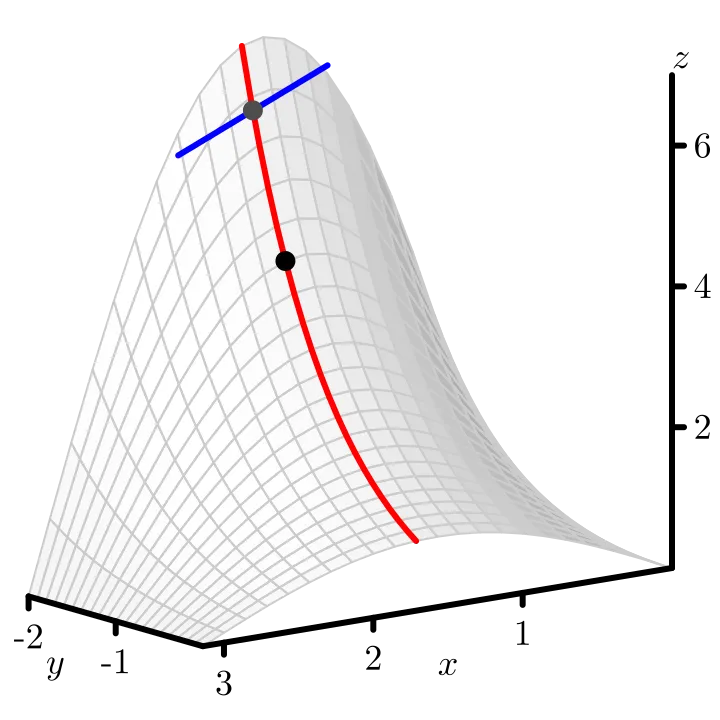
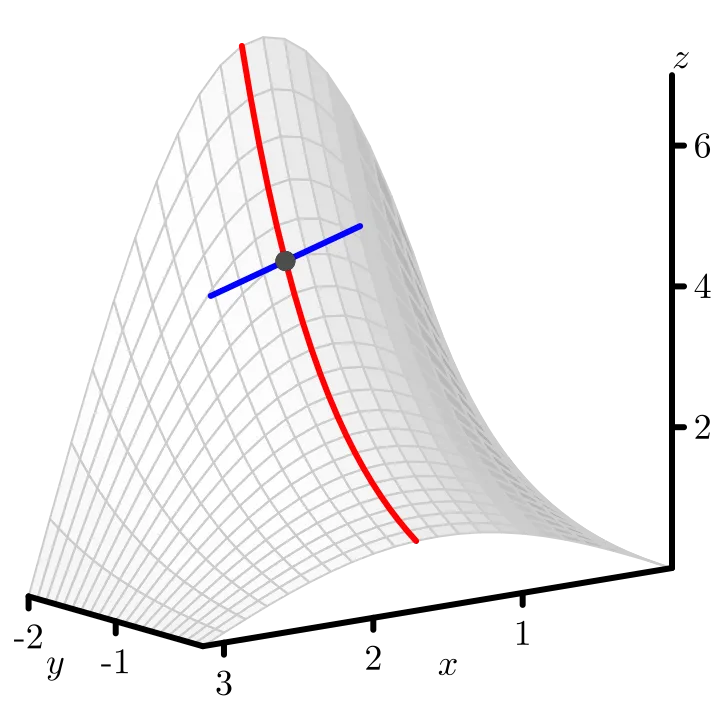
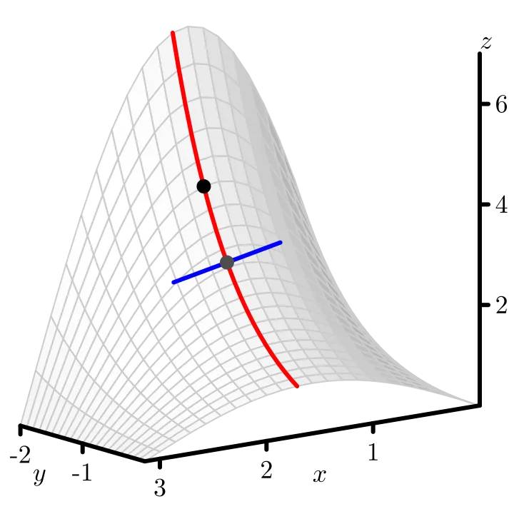
Based on Figure , is positive or negative? Why?
c. Determine the formula for and hence evaluate How does this value compare with your observations in (b)?
d. We know that measures the concavity of the trace, and that measures the concavity of the trace. What do you think the quantity measures?
e. On Figure , sketch the trace with and sketch three tangent lines whose slopes correspond to the value of for three different values of the middle of which is Is positive or negative? Why? What does measure?
Just as with the first-order partial derivatives, we can approximate second-order partial derivatives in the situation where we have only partial information about the function.
Activity
As we saw in Activity 10.2.5, the wind chill in degrees Fahrenheit, is a function of the wind speed, in miles per hour, and the air temperature, in degrees Fahrenheit. Some values of the wind chill are recorded in Table .
Table . Wind chill as a function of wind speed and temperature.
| -30 | -25 | -20 | -15 | -10 | -5 | 0 | 5 | 10 | 15 | 20 | |
|---|---|---|---|---|---|---|---|---|---|---|---|
| 5 | -46 | -40 | -34 | -28 | -22 | -16 | -11 | -5 | 1 | 7 | 13 |
| 10 | -53 | -47 | -41 | -35 | -28 | -22 | -16 | -10 | -4 | 3 | 9 |
| 15 | -58 | -51 | -45 | -39 | -32 | -26 | -19 | -13 | -7 | 0 | 6 |
| 20 | -61 | -55 | -48 | -42 | -35 | -29 | -22 | -15 | -9 | -2 | 4 |
| 25 | -64 | -58 | -51 | -44 | -37 | -31 | -24 | -17 | -11 | -4 | 3 |
| 30 | -67 | -60 | -53 | -46 | -39 | -33 | -26 | -19 | -12 | -5 | 1 |
| 35 | -69 | -62 | -55 | -48 | -41 | -34 | -27 | -21 | -14 | -7 | 0 |
| 40 | -71 | -64 | -57 | -50 | -43 | -36 | -29 | -22 | -15 | -8 | -1 |
- Estimate the partial derivatives and Use these results to estimate the second-order partial
- In a similar way, estimate the second-order partial
- Estimate the partial derivatives and and use your results to estimate the partial
- In a similar way, estimate the partial derivative
- Write several sentences that explain what the values and indicate regarding the behavior of
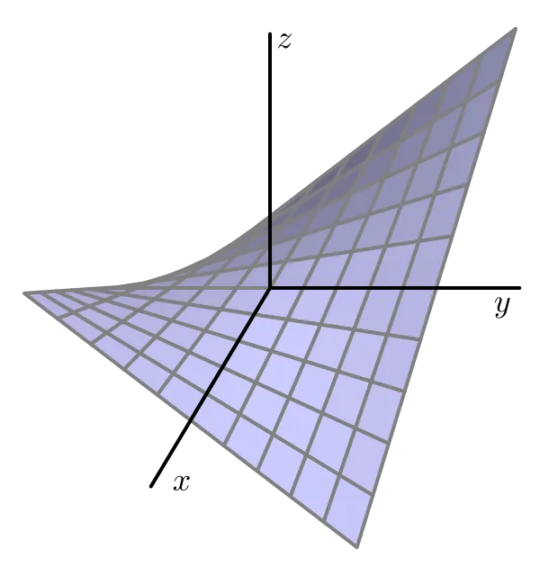
As we have found in Activities and Activity , we may think of as measuring the “twist” of the graph as we increase along a particular trace where is held constant. In the same way, measures how the graph twists as we increase If we remember that Clairaut's theorem tells us that we see that the amount of twisting is the same in both directions. This twisting is perhaps more easily seen in Figure , which shows the graph of for which
Summary
- There are four second-order partial derivatives of a function of two independent variables and
- The unmixed second-order partial derivatives, and tell us about the concavity of the traces. The mixed second-order partial derivatives, and tell us how the graph of twists.