Active Calculus · 10: Derivatives of Multivariable Functions

10.2: First-Order Partial Derivatives

Motivating Questions
  • How are the first-order partial derivatives of a function ff of the independent variables xx and yy defined?
  • Given a function ff of the independent variables xx and y,y\text{,} what do the first-order partial derivatives ∂f∂x\frac{\partial f}{\partial x} and ∂f∂y\frac{\partial f}{\partial y} tell us about f?f\text{?}

The derivative plays a central role in first semester calculus because it provides important information about a function. Thinking graphically, for instance, the derivative at a point tells us the slope of the tangent line to the graph at that point. In addition, the derivative at a point also provides the instantaneous rate of change of the function with respect to changes in the independent variable.

Now that we are investigating functions of two or more variables, we can still ask how fast the function is changing, though we have to be careful about what we mean. Thinking graphically again, we can try to measure how steep the graph of the function is in a particular direction. Alternatively, we may want to know how fast a function's output changes in response to a change in one of the inputs. Over the next few sections, we will develop tools for addressing issues such as these. Preview Activity 10.2.110.2.1 explores some issues with what we will come to call partial derivatives.

Preview Activity 10.2.110.2.1

Suppose we take out an $18,000 car loan at interest rate rr and we agree to pay off the loan in tt years. The monthly payment, in dollars, is

M(r,t)=1500r1−(1+r12)−12t. M(r,t) = \frac{1500r}{1-\left(1+\frac{r}{12}\right)^{-12t}}.

  1. What is the monthly payment if the interest rate is 3%3\% so that r=0.03,r = 0.03\text{,} and we pay the loan off in t=4t=4 years?
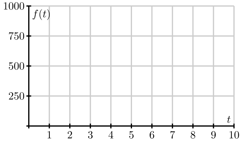
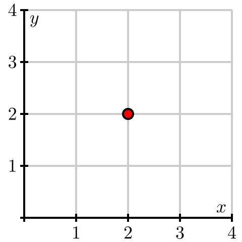
  2. Suppose the interest rate is fixed at 3%.3\%\text{.} Express MM as a function ff of tt alone using r=0.03.r=0.03\text{.} That is, let f(t)=M(0.03,t).f(t) = M(0.03, t)\text{.} Sketch the graph of ff on the left of Figure 10.2.110.2.1. Explain the meaning of the function f.f\text{.}
fig_10_2_preview_1.svg
fig_10_2_preview_2.svg
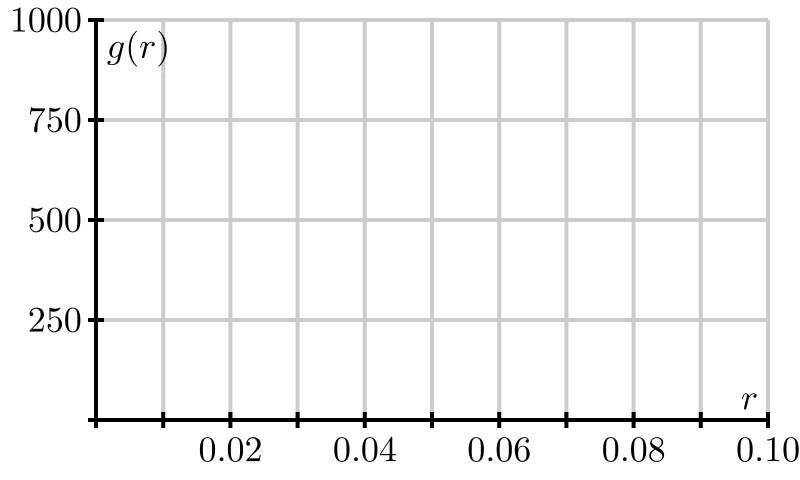
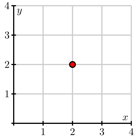
Figure 10.2.110.2.1. Left: Graphs f(t)=M(0.03,t).f(t)= M(0.03, t)\text{.} Right: Graph g(r)=M(r,4).g(r) = M(r,4)\text{.}
  1. Find the instantaneous rate of change f′(4)f'(4) and state the units on this quantity. What information does f′(4)f'(4) tell us about our car loan? What information does f′(4)f'(4) tell us about the graph you sketched in (b)?
  2. Express MM as a function of rr alone, using a fixed time of t=4.t=4\text{.} That is, let g(r)=M(r,4).g(r) = M(r, 4)\text{.} Sketch the graph of gg on the right of Figure 10.2.110.2.1. Explain the meaning of the function g.g\text{.}
  3. Find the instantaneous rate of change g′(0.03)g'(0.03) and state the units on this quantity. What information does g′(0.03)g'(0.03) tell us about our car loan? What information does g′(0.03)g'(0.03) tell us about the graph you sketched in (d)?

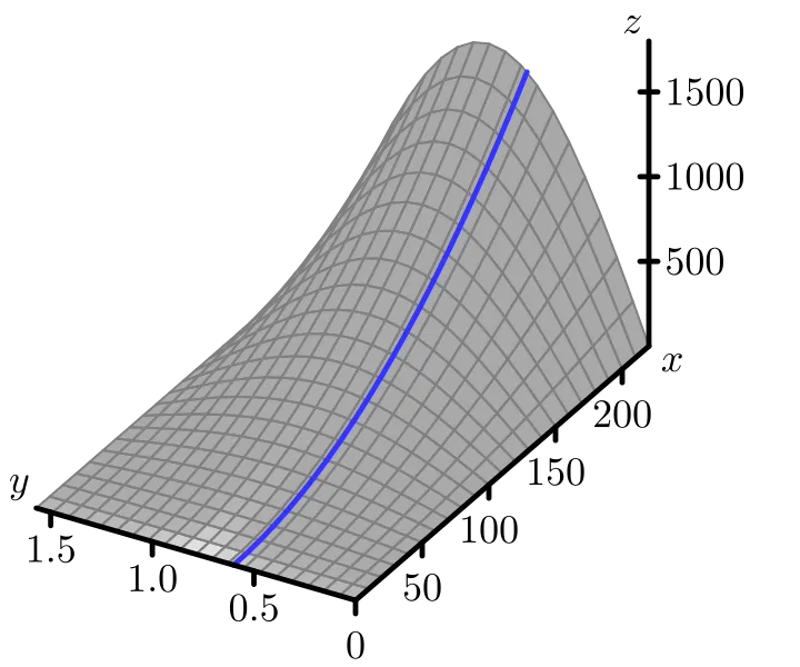
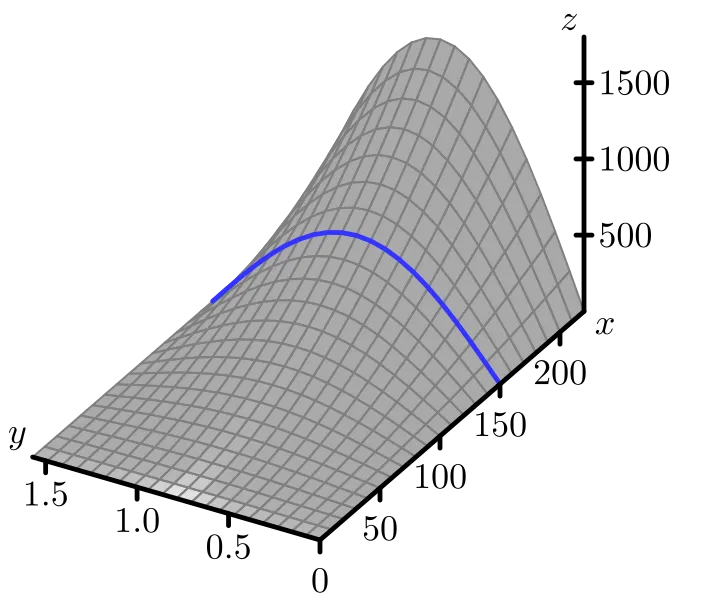
In Section 9.1, we studied the behavior of a function of two or more variables by considering the traces of the function. Recall that in one example, we considered the function ff defined by

f(x,y)=x2sin⁡(2y)32, f(x,y) = \frac{x^2 \sin(2 y)}{32},

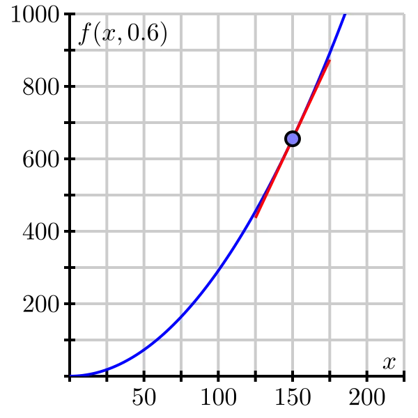
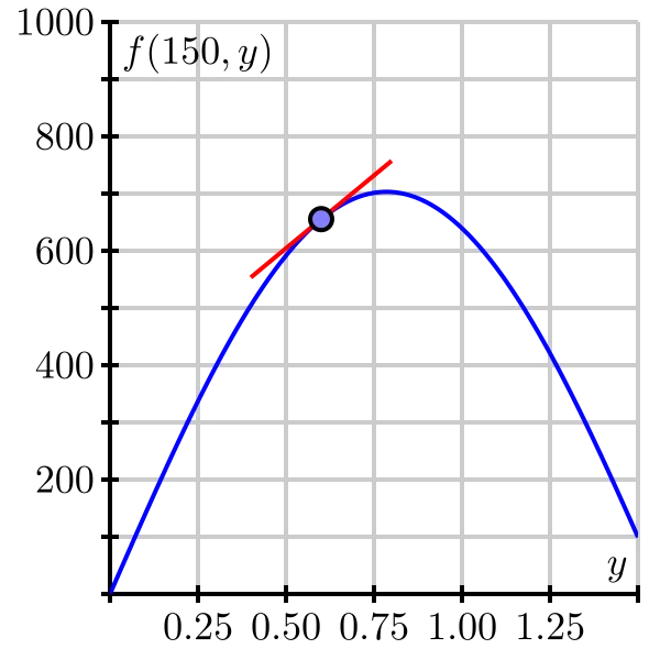
which measures the range, or horizontal distance, in feet, traveled by a projectile launched with an initial speed of xx feet per second at an angle yy radians to the horizontal. The graph of this function is given again on the left in Figure 10.2.210.2.2. Moreover, if we fix the angle y=0.6,y = 0.6\text{,} we may view the trace f(x,0.6)f(x,0.6) as a function of xx alone, as seen at right in Figure 10.2.210.2.2.

fig_10_2_trace_y_a.svg
fig_10_2_trace_y.svg
Figure 10.2.210.2.2. Left: The trace of z=x2sin⁡(2y)32z=\frac{x^2 \sin(2 y)}{32} with y=0.6.y = 0.6\text{.}

Since the trace is a one-variable function, we may consider its derivative just as we did in the first semester of calculus. With y=0.6,y=0.6\text{,} we have

f(x,0.6)=sin⁡(1.2)32x2, f(x,0.6) = \frac{\sin(1.2)}{32}x^2,

and therefore

ddx[f(x,0.6)]=sin⁡(1.2)16x. \frac{d}{dx}[f(x,0.6)] = \frac{\sin(1.2)}{16}x.

When x=150,x=150\text{,} this gives

ddx[f(x,0.6)]∣x=150=sin⁡(1.2)16150≈8.74 feet per feet per second, \frac{d}{dx}[f(x,0.6)]|_{x=150} = \frac{\sin(1.2)}{16}150 \approx 8.74~\mbox{feet per feet per second} ,

which gives the slope of the tangent line shown on the right of Figure 10.2.210.2.2. Thinking of this derivative as an instantaneous rate of change implies that if we increase the initial speed of the projectile by one foot per second, we expect the horizontal distance traveled to increase by approximately 8.74 feet if we hold the launch angle constant at 0.60.6 radians.

By holding yy fixed and differentiating with respect to x,x\text{,} we obtain the first-order partial derivative of ff with respect to xx. Denoting this partial derivative as fx,f_x\text{,} we have seen that

fx(150,0.6)=ddxf(x,0.6)∣x=150=lim⁡h→0f(150+h,0.6)−f(150,0.6)h. f_x(150, 0.6) = \frac{d}{dx}f(x,0.6)|_{x=150} = \lim_{h\to 0}\frac{f(150+h, 0.6) - f(150, 0.6)}{h}.

More generally, we have

fx(a,b)=lim⁡h→0f(a+h,b)−f(a,b)h, f_x(a,b) = \lim_{h\to0} \frac{f(a+h, b)-f(a,b)}{h},

provided this limit exists.

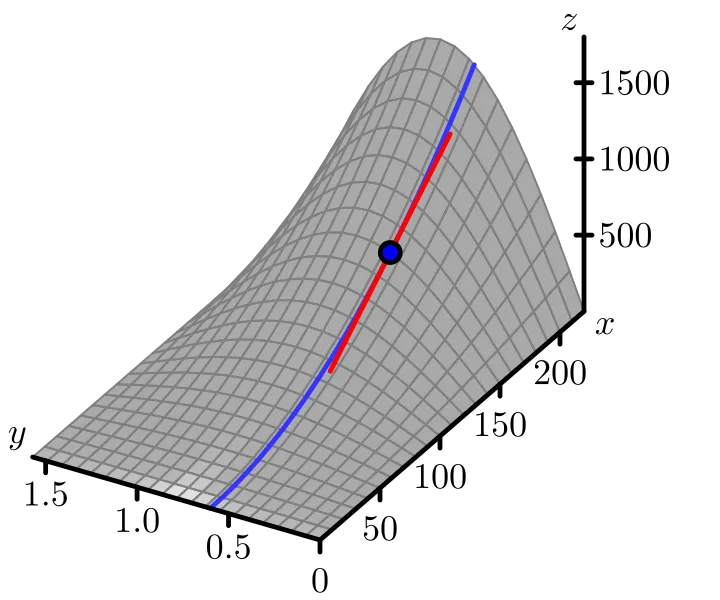
In the same way, we may obtain a trace by setting, say, x=150x=150 as shown in Figure 10.2.310.2.3.

fig_10_2_trace_x_a.svg
fig_10_2_trace_x.svg
Figure 10.2.310.2.3. The trace of z=x2sin⁡(2y)32z=\frac{x^2 \sin(2 y)}{32} with x=150.x = 150\text{.}

This gives

f(150,y)=150232sin⁡(2y), f(150, y) = \frac{150^2}{32}\sin(2y),

and therefore

ddy[f(150,y)]=150216cos⁡(2y). \frac{d}{dy}[f(150,y)] = \frac{150^2}{16}\cos(2y).

If we evaluate this quantity at y=0.6,y=0.6\text{,} we have

ddy[f(150,y)]∣y=0.6=150216cos⁡(1.2)≈509.5 feet per radian. \frac{d}{dy}[f(150,y)]|_{y=0.6} = \frac{150^2}{16}\cos(1.2) \approx 509.5 ~\mbox{feet per radian} .

Once again, the derivative gives the slope of the tangent line shown on the right in Figure 10.2.310.2.3. Thinking of the derivative as an instantaneous rate of change, we expect that the range of the projectile increases by 509.5 feet for every radian we increase the launch angle yy if we keep the initial speed of the projectile constant at 150 feet per second.

By holding xx fixed and differentiating with respect to y,y\text{,} we obtain the first-order partial derivative of ff with respect to yy. As before, we denote this partial derivative as fyf_y and write

fy(150,0.6)=ddyf(150,y)∣y=0.6=lim⁡h→0f(150,0.6+h)−f(150,0.6)h. f_y(150, 0.6) = \frac{d}{dy}f(150,y)|_{y=0.6} = \lim_{h\to 0}\frac{f(150, 0.6+h) - f(150, 0.6)}{h}.

As with the partial derivative with respect to x,x\text{,} we may express this quantity more generally at an arbitrary point (a,b).(a,b)\text{.} To recap, we have now arrived at the formal definition of the first-order partial derivatives of a function of two variables.

Definition 10.2.110.2.1

The first-order partial derivatives of ff with respect to xx and yy at a point (a,b)(a,b) are, respectively,

<spanclass="katex"><mathxmlns="http://www.w3.org/1998/Math/MathML"display="block"><semantics><mtablerowspacing="0.25em"columnalign="rightleft"columnspacing="0em"><mtr><mtd><mstylescriptlevel="0"displaystyle="true"><mrow><msub><mi>f</mi><mi>x</mi></msub><mostretchy="false">(</mo><mi>a</mi><moseparator="true">,</mo><mi>b</mi><mostretchy="false">)</mo></mrow></mstyle></mtd><mtd><mstylescriptlevel="0"displaystyle="true"><mrow><mrow></mrow><mo>=</mo><munder><mrow><mi>lim</mi><mo>⁡</mo></mrow><mrow><mi>h</mi><mo>→</mo><mn>0</mn></mrow></munder><mfrac><mrow><mi>f</mi><mostretchy="false">(</mo><mi>a</mi><mo>+</mo><mi>h</mi><moseparator="true">,</mo><mi>b</mi><mostretchy="false">)</mo><mo>−</mo><mi>f</mi><mostretchy="false">(</mo><mi>a</mi><moseparator="true">,</mo><mi>b</mi><mostretchy="false">)</mo></mrow><mi>h</mi></mfrac><moseparator="true">,</mo><mtext> and</mtext></mrow></mstyle></mtd></mtr><mtr><mtd><mstylescriptlevel="0"displaystyle="true"><mrow><msub><mi>f</mi><mi>y</mi></msub><mostretchy="false">(</mo><mi>a</mi><moseparator="true">,</mo><mi>b</mi><mostretchy="false">)</mo></mrow></mstyle></mtd><mtd><mstylescriptlevel="0"displaystyle="true"><mrow><mrow></mrow><mo>=</mo><munder><mrow><mi>lim</mi><mo>⁡</mo></mrow><mrow><mi>h</mi><mo>→</mo><mn>0</mn></mrow></munder><mfrac><mrow><mi>f</mi><mostretchy="false">(</mo><mi>a</mi><moseparator="true">,</mo><mi>b</mi><mo>+</mo><mi>h</mi><mostretchy="false">)</mo><mo>−</mo><mi>f</mi><mostretchy="false">(</mo><mi>a</mi><moseparator="true">,</mo><mi>b</mi><mostretchy="false">)</mo></mrow><mi>h</mi></mfrac><moseparator="true">,</mo></mrow></mstyle></mtd></mtr></mtable><annotationencoding="application/x−tex">fx(a,b)=lim⁡h→0f(a+h,b)−f(a,b)h, andfy(a,b)=lim⁡h→0f(a,b+h)−f(a,b)h,</annotation></semantics></math></span><span class="katex"><math xmlns="http://www.w3.org/1998/Math/MathML" display="block"><semantics><mtable rowspacing="0.25em" columnalign="right left" columnspacing="0em"><mtr><mtd><mstyle scriptlevel="0" displaystyle="true"><mrow><msub><mi>f</mi><mi>x</mi></msub><mo stretchy="false">(</mo><mi>a</mi><mo separator="true">,</mo><mi>b</mi><mo stretchy="false">)</mo></mrow></mstyle></mtd><mtd><mstyle scriptlevel="0" displaystyle="true"><mrow><mrow></mrow><mo>=</mo><munder><mrow><mi>lim</mi><mo>⁡</mo></mrow><mrow><mi>h</mi><mo>→</mo><mn>0</mn></mrow></munder><mfrac><mrow><mi>f</mi><mo stretchy="false">(</mo><mi>a</mi><mo>+</mo><mi>h</mi><mo separator="true">,</mo><mi>b</mi><mo stretchy="false">)</mo><mo>−</mo><mi>f</mi><mo stretchy="false">(</mo><mi>a</mi><mo separator="true">,</mo><mi>b</mi><mo stretchy="false">)</mo></mrow><mi>h</mi></mfrac><mo separator="true">,</mo><mtext> and</mtext></mrow></mstyle></mtd></mtr><mtr><mtd><mstyle scriptlevel="0" displaystyle="true"><mrow><msub><mi>f</mi><mi>y</mi></msub><mo stretchy="false">(</mo><mi>a</mi><mo separator="true">,</mo><mi>b</mi><mo stretchy="false">)</mo></mrow></mstyle></mtd><mtd><mstyle scriptlevel="0" displaystyle="true"><mrow><mrow></mrow><mo>=</mo><munder><mrow><mi>lim</mi><mo>⁡</mo></mrow><mrow><mi>h</mi><mo>→</mo><mn>0</mn></mrow></munder><mfrac><mrow><mi>f</mi><mo stretchy="false">(</mo><mi>a</mi><mo separator="true">,</mo><mi>b</mi><mo>+</mo><mi>h</mi><mo stretchy="false">)</mo><mo>−</mo><mi>f</mi><mo stretchy="false">(</mo><mi>a</mi><mo separator="true">,</mo><mi>b</mi><mo stretchy="false">)</mo></mrow><mi>h</mi></mfrac><mo separator="true">,</mo></mrow></mstyle></mtd></mtr></mtable><annotation encoding="application/x-tex">\begin{align*} f_x(a,b) & = \lim_{h \to 0} \frac{f(a+h,b)-f(a,b)}{h}, \ \mbox{and}\\[4pt] f_y(a,b) & = \lim_{h \to 0} \frac{f(a,b+h)-f(a,b)}{h}, \end{align*}</annotation></semantics></math></span>

provided the limits exist.

Activity 10.2.210.2.2

Consider the function ff defined by

f(x,y)=xy2x+1 f(x,y) = \frac{xy^2}{x+1}

at the point (1,2).(1,2)\text{.}

  1. Write the trace f(x,2)f(x,2) at the fixed value y=2.y=2\text{.} On the left side of Figure 10.2.410.2.4, draw the graph of the trace with y=2y=2 around the point where x=1,x=1\text{,} indicating the scale and labels on the axes. Also, sketch the tangent line at the point x=1.x=1\text{.}
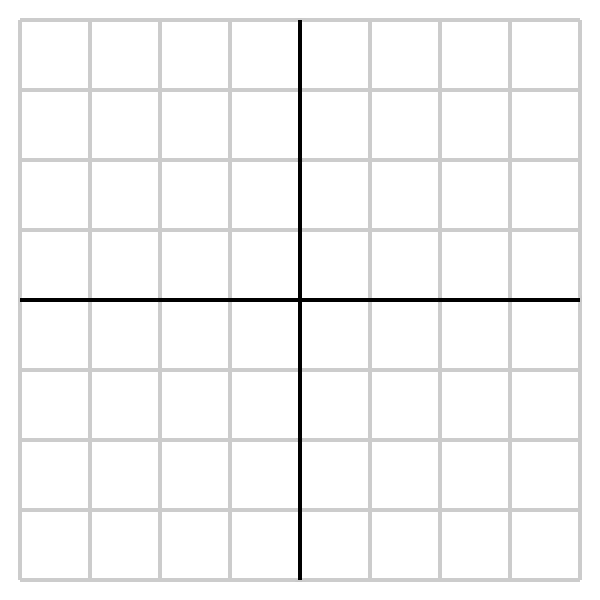
fig_10_2_empty.svg
fig_10_2_empty.svg
Figure 10.2.410.2.4. Traces of f(x,y)=xy2x+1.f(x,y) = \frac{xy^2}{x+1}\text{.}
  1. Find the partial derivative fx(1,2)f_x(1,2) and relate its value to the sketch you just made.
  2. Write the trace f(1,y)f(1,y) at the fixed value x=1.x=1\text{.} On the right side of Figure 10.2.510.2.5, draw the graph of the trace with x=1x=1 indicating the scale and labels on the axes. Also, sketch the tangent line at the point y=2.y=2\text{.}
  3. Find the partial derivative fy(1,2)f_y(1,2) and relate its value to the sketch you just made.

As these examples show, each partial derivative at a point arises as the derivative of a one-variable function defined by fixing one of the coordinates. In addition, we may consider each partial derivative as defining a new function of the point (x,y),(x,y)\text{,} just as the derivative f′(x)f'(x) defines a new function of xx in single-variable calculus. Due to the connection between one-variable derivatives and partial derivatives, we will often use Leibniz-style notation to denote partial derivatives by writing

∂f∂x(a,b)=fx(a,b), and ∂f∂y(a,b)=fy(a,b). \frac{\partial f}{\partial x}(a, b) = f_x(a,b), \ \mbox{and} \ \frac{\partial f}{\partial y}(a, b) = f_y(a,b).

To calculate the partial derivative fx,f_x\text{,} we hold yy fixed and thus we treat yy as a constant. In Leibniz notation, observe that

∂∂x(x)=1 and ∂∂x(y)=0. \frac{\partial }{\partial x} (x) = 1 \ \mbox{and} \ \frac{\partial }{\partial x}(y) = 0.

To see the contrast between how we calculate single variable derivatives and partial derivatives, and the difference between the notations ddx[ ]\frac{d}{dx}[ \ ] and ∂∂x[ ],\frac{\partial}{\partial x}[ \ ]\text{,} observe that

<spanclass="katex"><mathxmlns="http://www.w3.org/1998/Math/MathML"display="block"><semantics><mtablerowspacing="0.25em"columnalign="rightleft"columnspacing="0em"><mtr><mtd><mstylescriptlevel="0"displaystyle="true"><mrow></mrow></mstyle></mtd><mtd><mstylescriptlevel="0"displaystyle="true"><mrow><mrow></mrow><mfrac><mi>d</mi><mrow><mi>d</mi><mi>x</mi></mrow></mfrac><mostretchy="false">[</mo><mn>3</mn><msup><mi>x</mi><mn>2</mn></msup><mo>−</mo><mn>2</mn><mi>x</mi><mo>+</mo><mn>3</mn><mostretchy="false">]</mo><mo>=</mo><mn>3</mn><mfrac><mi>d</mi><mrow><mi>d</mi><mi>x</mi></mrow></mfrac><mostretchy="false">[</mo><msup><mi>x</mi><mn>2</mn></msup><mostretchy="false">]</mo><mo>−</mo><mn>2</mn><mfrac><mi>d</mi><mrow><mi>d</mi><mi>x</mi></mrow></mfrac><mostretchy="false">[</mo><mi>x</mi><mostretchy="false">]</mo><mo>+</mo><mfrac><mi>d</mi><mrow><mi>d</mi><mi>x</mi></mrow></mfrac><mostretchy="false">[</mo><mn>3</mn><mostretchy="false">]</mo><mo>=</mo><mn>3</mn><mo>⋅</mo><mn>2</mn><mi>x</mi><mo>−</mo><mn>2</mn><moseparator="true">,</mo></mrow></mstyle></mtd></mtr><mtr><mtd><mstylescriptlevel="0"displaystyle="true"><mtext>and </mtext></mstyle></mtd><mtd><mstylescriptlevel="0"displaystyle="true"><mrow><mrow></mrow><mfrac><mimathvariant="normal">∂</mi><mrow><mimathvariant="normal">∂</mi><mi>x</mi></mrow></mfrac><mostretchy="false">[</mo><msup><mi>x</mi><mn>2</mn></msup><mi>y</mi><mo>−</mo><mi>x</mi><mi>y</mi><mo>+</mo><mn>2</mn><mi>y</mi><mostretchy="false">]</mo><mo>=</mo><mi>y</mi><mfrac><mimathvariant="normal">∂</mi><mrow><mimathvariant="normal">∂</mi><mi>x</mi></mrow></mfrac><mostretchy="false">[</mo><msup><mi>x</mi><mn>2</mn></msup><mostretchy="false">]</mo><mo>−</mo><mi>y</mi><mfrac><mimathvariant="normal">∂</mi><mrow><mimathvariant="normal">∂</mi><mi>x</mi></mrow></mfrac><mostretchy="false">[</mo><mi>x</mi><mostretchy="false">]</mo><mo>+</mo><mfrac><mimathvariant="normal">∂</mi><mrow><mimathvariant="normal">∂</mi><mi>x</mi></mrow></mfrac><mostretchy="false">[</mo><mn>2</mn><mi>y</mi><mostretchy="false">]</mo><mo>=</mo><mi>y</mi><mo>⋅</mo><mn>2</mn><mi>x</mi><mo>−</mo><mi>y</mi></mrow></mstyle></mtd></mtr></mtable><annotationencoding="application/x−tex">ddx[3x2−2x+3]=3ddx[x2]−2ddx[x]+ddx[3]=3⋅2x−2,and ∂∂x[x2y−xy+2y]=y∂∂x[x2]−y∂∂x[x]+∂∂x[2y]=y⋅2x−y</annotation></semantics></math></span><span class="katex"><math xmlns="http://www.w3.org/1998/Math/MathML" display="block"><semantics><mtable rowspacing="0.25em" columnalign="right left" columnspacing="0em"><mtr><mtd><mstyle scriptlevel="0" displaystyle="true"><mrow></mrow></mstyle></mtd><mtd><mstyle scriptlevel="0" displaystyle="true"><mrow><mrow></mrow><mfrac><mi>d</mi><mrow><mi>d</mi><mi>x</mi></mrow></mfrac><mo stretchy="false">[</mo><mn>3</mn><msup><mi>x</mi><mn>2</mn></msup><mo>−</mo><mn>2</mn><mi>x</mi><mo>+</mo><mn>3</mn><mo stretchy="false">]</mo><mo>=</mo><mn>3</mn><mfrac><mi>d</mi><mrow><mi>d</mi><mi>x</mi></mrow></mfrac><mo stretchy="false">[</mo><msup><mi>x</mi><mn>2</mn></msup><mo stretchy="false">]</mo><mo>−</mo><mn>2</mn><mfrac><mi>d</mi><mrow><mi>d</mi><mi>x</mi></mrow></mfrac><mo stretchy="false">[</mo><mi>x</mi><mo stretchy="false">]</mo><mo>+</mo><mfrac><mi>d</mi><mrow><mi>d</mi><mi>x</mi></mrow></mfrac><mo stretchy="false">[</mo><mn>3</mn><mo stretchy="false">]</mo><mo>=</mo><mn>3</mn><mo>⋅</mo><mn>2</mn><mi>x</mi><mo>−</mo><mn>2</mn><mo separator="true">,</mo></mrow></mstyle></mtd></mtr><mtr><mtd><mstyle scriptlevel="0" displaystyle="true"><mtext>and </mtext></mstyle></mtd><mtd><mstyle scriptlevel="0" displaystyle="true"><mrow><mrow></mrow><mfrac><mi mathvariant="normal">∂</mi><mrow><mi mathvariant="normal">∂</mi><mi>x</mi></mrow></mfrac><mo stretchy="false">[</mo><msup><mi>x</mi><mn>2</mn></msup><mi>y</mi><mo>−</mo><mi>x</mi><mi>y</mi><mo>+</mo><mn>2</mn><mi>y</mi><mo stretchy="false">]</mo><mo>=</mo><mi>y</mi><mfrac><mi mathvariant="normal">∂</mi><mrow><mi mathvariant="normal">∂</mi><mi>x</mi></mrow></mfrac><mo stretchy="false">[</mo><msup><mi>x</mi><mn>2</mn></msup><mo stretchy="false">]</mo><mo>−</mo><mi>y</mi><mfrac><mi mathvariant="normal">∂</mi><mrow><mi mathvariant="normal">∂</mi><mi>x</mi></mrow></mfrac><mo stretchy="false">[</mo><mi>x</mi><mo stretchy="false">]</mo><mo>+</mo><mfrac><mi mathvariant="normal">∂</mi><mrow><mi mathvariant="normal">∂</mi><mi>x</mi></mrow></mfrac><mo stretchy="false">[</mo><mn>2</mn><mi>y</mi><mo stretchy="false">]</mo><mo>=</mo><mi>y</mi><mo>⋅</mo><mn>2</mn><mi>x</mi><mo>−</mo><mi>y</mi></mrow></mstyle></mtd></mtr></mtable><annotation encoding="application/x-tex">\begin{align*} & \frac{d}{dx}[3x^2 - 2x + 3] = 3\frac{d}{dx}[x^2] - 2\frac{d}{dx}[x] + \frac{d}{dx}[3] = 3\cdot 2x - 2,\\[4pt] \mbox{and} \ & \frac{\partial}{\partial x}[x^2y - xy + 2y] = y\frac{\partial}{\partial x}[x^2] - y\frac{\partial}{\partial x}[x] + \frac{\partial}{\partial x}[2y] = y\cdot 2x - y \end{align*}</annotation></semantics></math></span>

Thus, computing partial derivatives is straightforward: we use the standard rules of single variable calculus, but do so while holding one (or more) of the variables constant.

Activity 10.2.310.2.3
  1. If f(x,y)=3x3−2x2y5,f(x,y) = 3x^3 - 2x^2y^5\text{,} find the partial derivatives fxf_x and fy.f_y\text{.}
  2. If f(x,y)=xy2x+1,f(x,y) = \displaystyle\frac{xy^2}{x+1}\text{,} find the partial derivatives fxf_x and fy.f_y\text{.}
  3. If g(r,s)=rscos⁡(r),g(r,s) = rs\cos(r)\text{,} find the partial derivatives grg_r and gs.g_s\text{.}
  4. Assuming f(w,x,y)=(6w+1)cos⁡(3x2+4xy3+y),f(w,x,y) = (6w+1)\cos(3x^2+4xy^3+y)\text{,} find the partial derivatives fw,f_w\text{,} fx,f_x\text{,} and fy.f_y\text{.}
  5. Find all possible first-order partial derivatives of q(x,t,z)=x2tz31+x2.q(x,t,z) = \displaystyle \frac{x2^tz^3}{1+x^2}.

Interpretations of First-Order Partial Derivatives

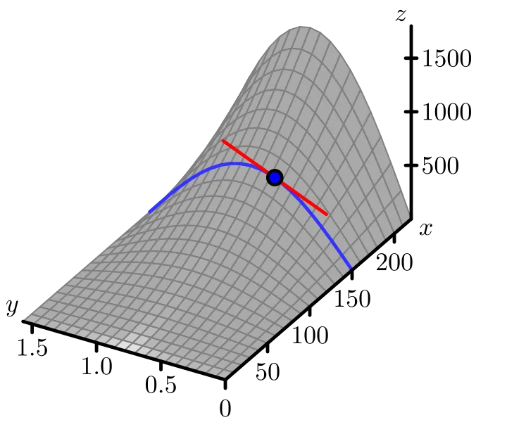
Recall that the derivative of a single variable function has a geometric interpretation as the slope of the line tangent to the graph at a given point. Similarly, we have seen that the partial derivatives measure the slope of a line tangent to a trace of a function of two variables as shown in Figure 10.2.510.2.5.

fig_10_2_trace_tangent_y.svg
fig_10_2_trace_tangent_x.svg
Figure 10.2.510.2.5. Tangent lines to two traces of the distance function.

Now we consider the first-order partial derivatives in context. Recall that the difference quotient f(a+h)−f(a)h\frac{f(a+h)-f(a)}{h} for a function ff of a single variable xx at a point where x=ax=a tells us the average rate of change of ff over the interval [a,a+h],[a,a+h]\text{,} while the derivative f′(a)f'(a) tells us the instantaneous rate of change of ff at x=a.x=a\text{.} We can use these same concepts to explain the meanings of the partial derivatives in context.

Activity 10.2.410.2.4

The speed of sound CC traveling through ocean water is a function of temperature, salinity and depth. It may be modeled by the function

C=1449.2+4.6T−0.055T2+0.00029T3+(1.34−0.01T)(S−35)+0.016D. C=1449.2+4.6T-0.055T^2+0.00029T^3+(1.34-0.01T)(S-35)+0.016D.

Here CC is the speed of sound in meters/second, TT is the temperature in degrees Celsius, SS is the salinity in grams/liter of water, and DD is the depth below the ocean surface in meters.

  1. State the units in which each of the partial derivatives, CT,C_T\text{,} CSC_S and CD,C_D\text{,} are expressed and explain the physical meaning of each.
  2. Find the partial derivatives CT,C_T\text{,} CSC_S and CD.C_D\text{.}
  3. Evaluate each of the three partial derivatives at the point where T=10,T=10\text{,} S=35S=35 and D=100.D=100\text{.} What does the sign of each partial derivatives tell us about the behavior of the function CC at the point (10,35,100)?(10,35, 100)\text{?}

Using tables and contours to estimate partial derivatives

Remember that functions of two variables are often represented as either a table of data or a contour plot. In single variable calculus, we saw how we can use the difference quotient to approximate derivatives if, instead of an algebraic formula, we only know the value of the function at a few points. The same idea applies to partial derivatives.

Activity 10.2.510.2.5

The wind chill, as frequently reported, is a measure of how cold it feels outside when the wind is blowing. In Table 10.2.110.2.1, the wind chill w,w\text{,} measured in degrees Fahrenheit, is a function of the wind speed v,v\text{,} measured in miles per hour, and the ambient air temperature T,T\text{,} also measured in degrees Fahrenheit. We thus view ww as being of the form w=w(v,T).w = w(v, T)\text{.}

Table 10.2.110.2.1. Wind chill as a function of wind speed and temperature.
v\Tv \backslash T −30-30 −25-25 −20-20 −15-15 −10-10 −5-5 00 55 1010 1515 2020
55 −46-46 −40-40 −34-34 −28-28 −22-22 −16-16 −11-11 −5-5 11 77 1313
1010 −53-53 −47-47 −41-41 −35-35 −28-28 −22-22 −16-16 −10-10 −4-4 33 99
1515 −58-58 −51-51 −45-45 −39-39 −32-32 −26-26 −19-19 −13-13 −7-7 00 66
2020 −61-61 −55-55 −48-48 −42-42 −35-35 −29-29 −22-22 −15-15 −9-9 −2-2 44
2525 −64-64 −58-58 −51-51 −44-44 −37-37 −31-31 −24-24 −17-17 −11-11 −4-4 33
3030 −67-67 −60-60 −53-53 −46-46 −39-39 −33-33 −26-26 −19-19 −12-12 −5-5 11
3535 −69-69 −62-62 −55-55 −48-48 −41-41 −34-34 −27-27 −21-21 −14-14 −7-7 00
4040 −71-71 −64-64 −57-57 −50-50 −43-43 −36-36 −29-29 −22-22 −15-15 −8-8 −1-1
  1. Estimate the partial derivative wv(20,−10).w_v(20,-10)\text{.} What are the units on this quantity and what does it mean? (Recall that we can estimate a partial derivative of a single variable function ff using the symmetric difference quotient f(x+h)−f(x−h)2h\frac{f(x+h)-f(x-h)}{2h} for small values of h.h\text{.} A partial derivative is a derivative of an appropriate trace.)
  2. Estimate the partial derivative wT(20,−10).w_T(20,-10)\text{.} What are the units on this quantity and what does it mean?
  3. Use your results to estimate the wind chill w(18,−10).w(18, -10)\text{.} (Recall from single variable calculus that for a function ff of x,x\text{,} f(x+h)≈f(x)+hf′(x).f(x+h) \approx f(x) + hf'(x)\text{.})
  4. Use your results to estimate the wind chill w(20,−12).w(20, -12)\text{.}
  5. Consider how you might combine your previous results to estimate the wind chill w(18,−12).w(18, -12)\text{.} Explain your process.
Activity 10.2.610.2.6

Shown below in Figure 10.2.610.2.6 is a contour plot of a function f.f\text{.} The values of the function on a few of the contours are indicated to the left of the figure.
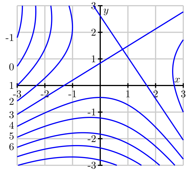
fig_10_2_activity_contours.svg
Figure 10.2.610.2.6. A contour plot of f.f\text{.}
  1. Estimate the partial derivative fx(−2,−1).f_x(-2,-1)\text{.} (Hint: How can you find values of ff that are of the form f(−2+h)f(-2+h) and f(−2−h)f(-2-h) so that you can use a symmetric difference quotient?)
  2. Estimate the partial derivative fy(−2,−1).f_y(-2,-1)\text{.}
  3. Estimate the partial derivatives fx(−1,2)f_x(-1,2) and fy(−1,2).f_y(-1,2)\text{.}
  4. Locate, if possible, one point (x,y)(x,y) where fx(x,y)=0.f_x(x,y)= 0\text{.}
  5. Locate, if possible, one point (x,y)(x,y) where fx(x,y)<0.f_x(x,y)\lt 0\text{.}
  6. Locate, if possible, one point (x,y)(x,y) where fy(x,y)>0.f_y(x,y)>0\text{.}
  7. Suppose you have a different function g,g\text{,} and you know that g(2,2)=4,g(2,2) = 4\text{,} gx(2,2)>0,g_x(2,2) > 0\text{,} and gy(2,2)>0.g_y(2,2) > 0\text{.} Using this information, sketch a possibility for the contour g(x,y)=4g(x,y)=4 passing through (2,2)(2,2) on the left side of Figure 10.2.710.2.7. Then include possible contours g(x,y)=3g(x,y) = 3 and g(x,y)=5.g(x,y) = 5\text{.}
fig_10_2_activity_grad.svg
fig_10_2_activity_grad-1.svg
Figure 10.2.710.2.7. Plots for contours of gg and h.h\text{.}
  1. Suppose you have yet another function h,h\text{,} and you know that h(2,2)=4,h(2,2) = 4\text{,} hx(2,2)<0,h_x(2,2) \lt 0\text{,} and hy(2,2)>0.h_y(2,2) > 0\text{.} Using this information, sketch a possible contour h(x,y)=4h(x,y)=4 passing through (2,2)(2,2) on the right side of Figure 10.2.910.2.9. Then include possible contours h(x,y)=3h(x,y) = 3 and h(x,y)=5.h(x,y) = 5\text{.}

Summary

  • If f=f(x,y)f=f(x,y) is a function of two variables, there are two first order partial derivatives of f:f\text{:} the partial derivative of ff with respect to x,x\text{,}
    ∂f∂x(x,y)=fx(x,y)=lim⁡h→0f(x+h,y)−f(x,y)h, \frac{\partial f}{\partial x}(x,y) = f_x(x,y) = \lim_{h \to 0} \frac{f(x+h,y) - f(x,y)}{h},

    and the partial derivative of ff with respect to y,y\text{,}

    ∂f∂y(x,y)=fy(x,y)=lim⁡h→0f(x,y+h)−f(x,y)h, \frac{\partial f}{\partial y}(x,y) = f_y(x,y) = \lim_{h \to 0} \frac{f(x,y+h) - f(x,y)}{h},

    where each partial derivative exists only at those points (x,y)(x,y) for which the limit exists.

  • The partial derivative fx(a,b)f_x(a,b) tells us the instantaneous rate of change of ff with respect to xx at (x,y)=(a,b)(x,y) = (a,b) when yy is fixed at b.b\text{.} Geometrically, the partial derivative fx(a,b)f_x(a,b) tells us the slope of the line tangent to the y=by=b trace of the function ff at the point (a,b,f(a,b)).(a,b,f(a,b))\text{.}
  • The partial derivative fy(a,b)f_y(a,b) tells us the instantaneous rate of change of ff with respect to yy at (x,y)=(a,b)(x,y) = (a,b) when xx is fixed at a.a\text{.} Geometrically, the partial derivative fy(a,b)f_y(a,b) tells us the slope of the line tangent to the x=ax=a trace of the function ff at the point (a,b,f(a,b)).(a,b,f(a,b))\text{.}

Credit and licence

This page titled 10.2: First-Order Partial Derivatives was last modified on Wed, 09 Nov 2022 21:17:06 GMT and is shared under a CC BY-SA 4.0 license and was authored, remixed, and/or curated by Matthew Boelkins, David Austin, and Steven Schlicker ( ScholarWorks @Grand Valley State University ) via source content that was edited to the style and standards of the LibreTexts platform.

Source: https://math.libretexts.org/Bookshelves/Calculus/Active_Calculus_(Boelkins_et_al.)/10%3A_Derivatives_of_Multivariable_Functions/10.02%3A_First-Order_Partial_Derivatives

Licence: CC BY-SA 4.0 (creativecommons.org/licenses/by-sa/4.0/). You may share and adapt it under the same licence, with this credit. WorldClass adapted the formatting only: the text is the authors', with interactive parts and links to other sites left out.

Build status · Flash Infinity AI™ is a trademark of AI-Flash Inc.. WorldClass is not affiliated with, approved or accredited by any exam board, curriculum provider or university unless a page says so.