Motivating Questions
- What does it mean for a function of two variables to be locally linear at a point?
- How do we find the equation of the plane tangent to a locally linear function at a point?
- What is the differential of a multivariable function of two variables and what are its uses?
One of the central concepts in single variable calculus is that the graph of a differentiable function, when viewed on a very small scale, looks like a line. We call this line the tangent line and measure its slope with the derivative. In this section, we will extend this concept to functions of several variables.
Let's see what happens when we look at the graph of a two-variable function on a small scale. To begin, let's consider the function defined by
whose graph is shown in Figure .
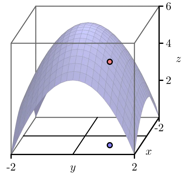
We choose to study the behavior of this function near the point In particular, we wish to view the graph on an increasingly small scale around this point, as shown in the two plots in Figure
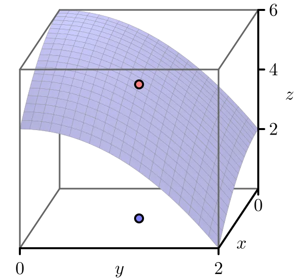
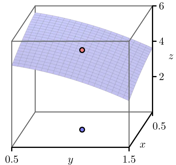
Just as the graph of a differentiable single-variable function looks like a line when viewed on a small scale, we see that the graph of this particular two-variable function looks like a plane, as seen in Figure . In the following preview activity, we explore how to find the equation of this plane.
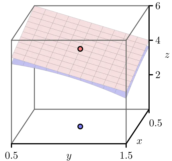
In what follows, we will also use the important fact 1 that the plane passing through may be expressed in the form where and are constants.
Preview Activity
Let and let
a. Evaluate and its partial derivatives at that is, find and
b. We know one point on the tangent plane; namely, the -value of the tangent plane agrees with the -value on the graph of at the point In other words, both the tangent plane and the graph of the function contain the point Use this observation to determine in the expression
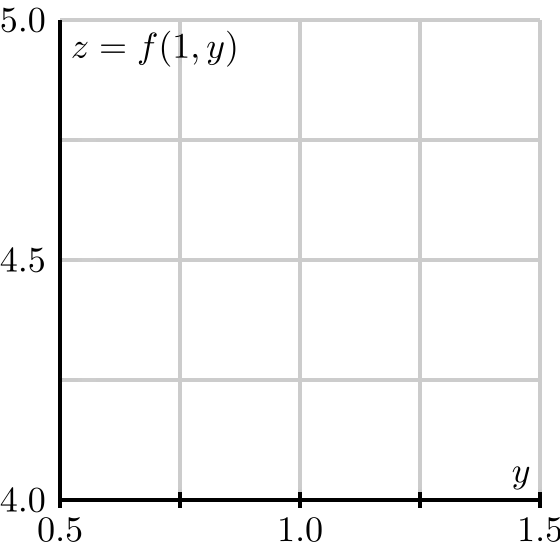
c. Sketch the traces of for and below in Figure .
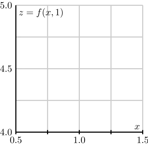
d. Determine the equation of the tangent line of the trace that you sketched in the previous part with (in the direction) at the point
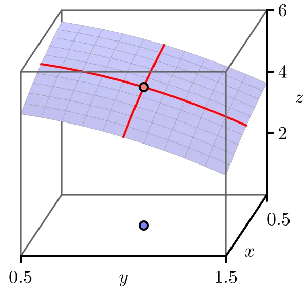
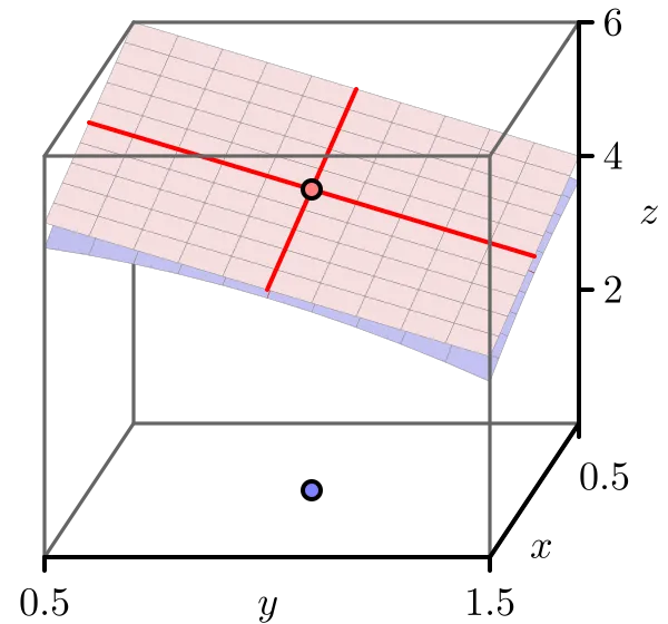
e. Figure shows the traces of the function and the traces of the tangent plane. Explain how the tangent line of the trace of whose equation you found in the last part of this activity, is related to the tangent plane. How does this observation help you determine the constant in the equation for the tangent plane (Hint: How do you think should be related to )
f. In a similar way to what you did in (d), determine the equation of the tangent line of the trace with at the point Explain how this tangent line is related to the tangent plane, and use this observation to determine the constant in the equation for the tangent plane (Hint: How do you think should be related to )
g. Finally, write the equation of the tangent plane to the graph of at the point
The Tangent Plane
Before stating the formula for the equation of the tangent plane at a point for a general function we need to discuss a technical condition. As we have noted, when we look at the graph of a single-variable function on a small scale near a point we expect to see a line; in this case, we say that is locally linear near since the graph looks like a linear function locally around Of course, there are functions, such as the absolute value function given by that are not locally linear at every point. In single-variable calculus, we learn that if the derivative of a function exists at a point, then the function is guaranteed to be locally linear there.
In a similar way, we say that a two-variable function is locally linear near provided that the graph of looks like a plane (its tangent plane) when viewed on a small scale near How can we tell when a function of two variables is locally linear at a point?
It is not unreasonable to expect that if and exist for some function at a point then is locally linear at This is not sufficient, however. As an example, consider the function defined by In Exercise you are asked to show that and both exist, but that is not locally linear at (see Figure 2). So the existence of the two first order partial derivatives at a point does not guarantee local linearity at that point.
It would take us too far afield to provide a rigorous discussion of differentiability of functions of more than one variable (see Exercise for a little more detail), so we will be content to define stronger, but more easily verified, conditions that ensure local linearity.
Differentiablity
If is a function of the independent variables and and both and exist and are continuous in an open disk containing the point then is continuously differentiable at
As a consequence, whenever a function is continuously differentiable at a point it follows that the function has a tangent plane at Viewed up close, the tangent plane and the function are then virtually indistinguishable. (We won't formally define differentiability of multivariable functions here, and for our purposes continuous differentiability is the only condition we will ever need to use. It is important to note that continuous differentiability is a stronger condition than differentiability. All of the results we encounter will apply to differentiable functions, and so also apply to continuously differentiable functions.) In addition, as in Preview Activity , we find the following general formula for the tangent plane.
The tangent plane
If has continuous first-order partial derivatives, then the equation of the plane tangent to the graph of at the point is
Important Note: As can be seen in Exercise .11, it is possible that and can exist for a function and so the plane exists even though is not locally linear at (because the graph of does not look linear when we zoom in around the point ). In such a case this plane is not tangent to the graph. Differentiability for a function of two variables implies the existence of a tangent plane, but the existence of the two first order partial derivatives of a function at a point does not imply differentiaility. This is quite different than what happens in single variable calculus.
Finally, one important note about the form of the equation for the tangent plane, Say, for example, that we have the particular tangent plane Observe that we can immediately read from this form that and furthermore, is the slope of the trace to both and the tangent plane in the -direction at In the same way, is the slope of the trace of both and the tangent plane in the -direction at
Activity
- Find the equation of the tangent plane to at the point Simplify as much as possible. Does the result surprise you? Explain.
- Find the equation of the tangent plane to at the point
Linearization
In single variable calculus, an important use of the tangent line is to approximate the value of a differentiable function. Near the point the tangent line to the graph of at is close to the graph of near as shown in Figure .
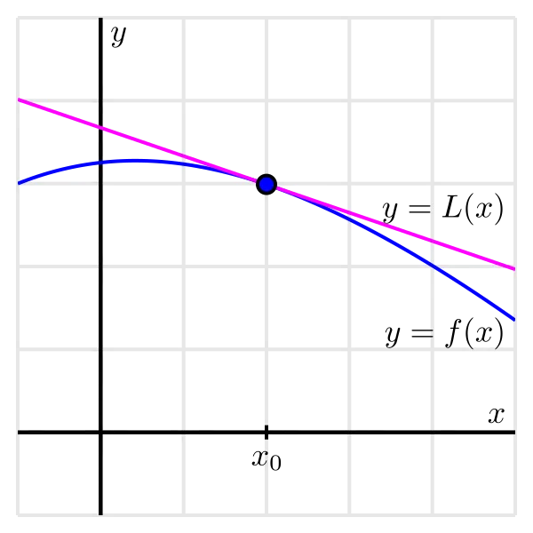
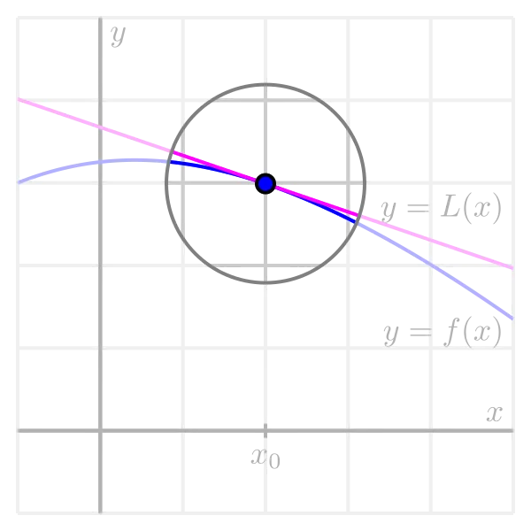
In this single-variable setting, we let denote the function whose graph is the tangent line, and thus
Furthermore, observe that near We call the linearization of
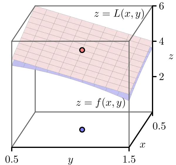
In the same way, the tangent plane to the graph of a differentiable function at a point provides a good approximation of near Here, we define the linearization, to be the two-variable function whose graph is the tangent plane, and thus
Finally, note that for points near This is illustrated in Figure .
Activity
In what follows, we find the linearization of several different functions that are given in algebraic, tabular, or graphical form.
a. Find the linearization for the function defined by
at the point Then use the linearization to estimate the value of
b. Table provides a collection of values of the wind chill in degrees Fahrenheit, as a function of wind speed, in miles per hour, and temperature, also in degrees Fahrenheit.
Table . Wind chill as a function of wind speed and temperature.
Use the data to first estimate the appropriate partial derivatives, and then find the linearization at the point Finally, use the linearization to estimate and Compare your results to what you obtained in Activity 10.2.5
c. Figure gives a contour plot of a continuously differentiable function
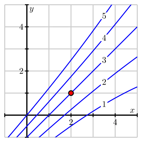
After estimating appropriate partial derivatives, determine the linearization at the point and use it to estimate and
Differentials
As we have seen, the linearization enables us to estimate the value of for points near the base point Sometimes, however, we are more interested in the change in as we move from the base point to another point
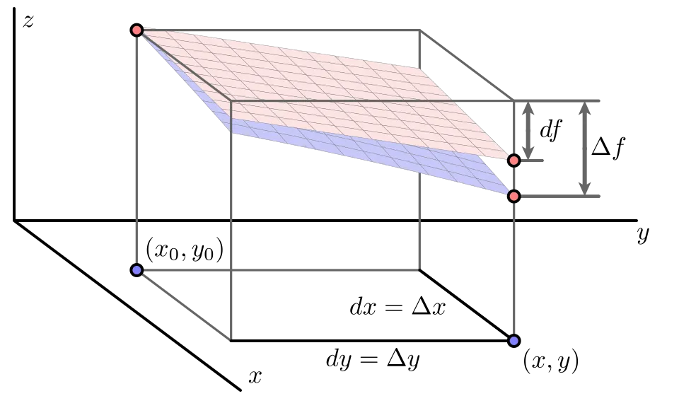
Figure 10.4.10\ illustrates this situation. Suppose we are at the point \((x_0,y_0)\text{,} and we know the value of at If we consider the displacement to a new point we would like to know how much the function has changed. We denote this change by where
A simple way to estimate the change is to approximate it by which represents the change in the linearization as we move from to This gives
For consistency, we will denote the change in the independent variables as and and thus
Expressed equivalently in Leibniz notation, we have
We call the quantities and differentials, and we think of them as measuring small changes in the quantities and Equations () and () express the relationship between these changes. Equation () resembles an important idea from single-variable calculus: when depends on it follows in the notation of differentials that
We will illustrate the use of differentials with an example.
Example
Suppose we have a machine that manufactures rectangles of width cm and height cm. However, the machine isn't perfect, and therefore the width could be off by cm and the height could be off by cm.
The area of the rectangle is
so that the area of a perfectly manufactured rectangle is square centimeters. Since the machine isn't perfect, we would like to know how much the area of a given manufactured rectangle could differ from the perfect rectangle. We will estimate the uncertainty in the area using (), and find that
Since and we have
That is, we estimate that the area in our rectangles could be off by as much as 10 square centimeters.
Activity
The questions in this activity explore the differential in several different contexts.
- Suppose that the elevation of a landscape is given by the function where we additionally know that and Assume that and are measured in miles in the easterly and northerly directions, respectively, from some base point Your GPS device says that you are currently at the point However, you know that the coordinates are only accurate to within units; that is, and Estimate the uncertainty in your elevation using differentials.
- The pressure, volume, and temperature of an ideal gas are related by the equation
where is measured in kilopascals, in liters, and in kelvin. Find the pressure when the volume is 12 liters and the temperature is 310 K. Use differentials to estimate the change in the pressure when the volume increases to 12.3 liters and the temperature decreases to 305 K.
- Refer to Table , the table of values of the wind chill in degrees Fahrenheit, as a function of temperature, also in degrees Fahrenheit, and wind speed, in miles per hour. Suppose your anemometer says the wind is blowing at miles per hour and your thermometer shows a reading of degrees. However, you know your thermometer is only accurate to within degrees and your anemometer is only accurate to within miles per hour. What is the wind chill based on your measurements? Estimate the uncertainty in your measurement of the wind chill.
Summary
- A function of two independent variables is locally linear at a point if the graph of looks like a plane as we zoom in on the graph around the point In this case, the equation of the tangent plane is given by
- The tangent plane when considered as a function, is called the linearization of a differentiable function at and may be used to estimate values of that is, for points near
- A function of two independent variables is differentiable at provided that both and exist and are continuous in an open disk containing the point
- The differential of a function is related to the differentials and by
We can use this relationship to approximate small changes in that result from small changes in and