Motivating Questions
- Given the graph of a function's derivative, how can we construct a completely accurate graph of the original function?
- How many antiderivatives does a given function have? What do those antiderivatives all have in common?
- Given a function how does the rule define a new function
A recurring theme in our discussion of differential calculus has been the question “Given information about the derivative of an unknown function how much information can we obtain about itself?” In Activity 1.8.3, the graph of was known (along with the value of at a single point) and we endeavored to sketch a possible graph of near the known point. In Example 3.1.2 — we investigated how the first derivative test enables us to use information about to determine where the original function is increasing and decreasing, as well as where has relative extreme values. If we know a formula or graph of by computing we can find where the original function is concave up and concave down. Thus, knowing and enables us to understand the shape of the graph of
We returned to this question in even more detail in Section 4.1. In that setting, we knew the instantaneous velocity of a moving object and worked to determine as much as possible about the object's position function. We found connections between the net signed area under the velocity function and the corresponding change in position of the function, and the Total Change Theorem further illuminated these connections between and showing that the total change in the value of over an interval is determined by the net signed area bounded by and the -axis on the same interval.
In what follows, we explore the situation where we possess an accurate graph of the derivative function along with a single value of the function From that information, we'd like to determine a graph of that shows where is increasing, decreasing, concave up, and concave down, and also provides an accurate function value at any point.
Preview Activity
Suppose that the following information is known about a function the graph of its derivative, is given in Figure . Further, assume that is piecewise linear (as pictured) and that for and Finally, it is given that
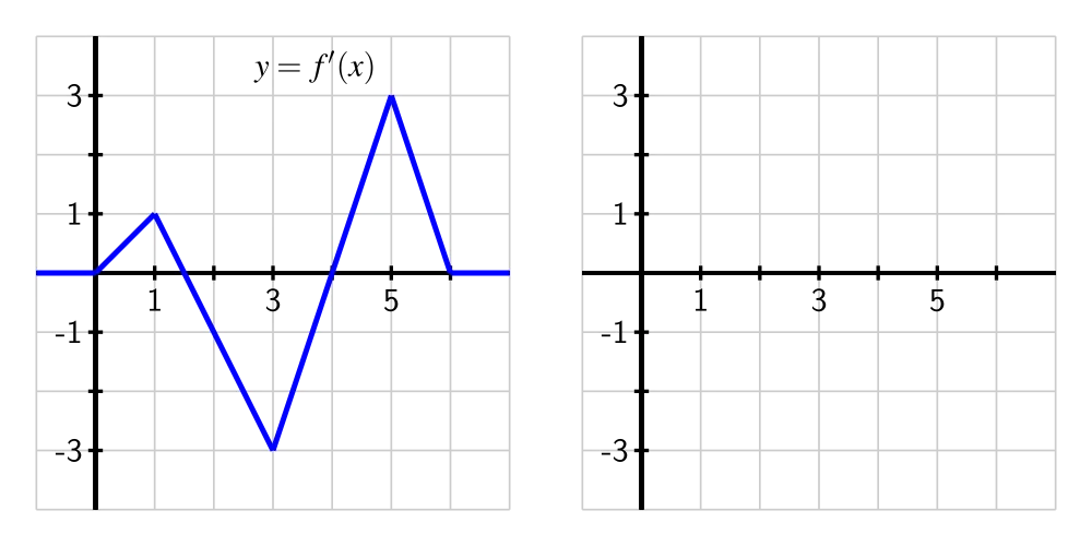
- On what interval(s) is an increasing function? On what intervals is decreasing?
- On what interval(s) is concave up? concave down?
- At what point(s) does have a relative minimum? a relative maximum?
- Recall that the Total Change Theorem tells us that
What is the exact value of
- Use the given information and similar reasoning to that in (d) to determine the exact value of and
- Based on your responses to all of the preceding questions, sketch a complete and accurate graph of on the axes provided, being sure to indicate the behavior of for and
Constructing the graph of an antiderivative
Preview Activity demonstrates that when we can find the exact area under the graph of a function on any given interval, it is possible to construct a graph of the function's antiderivative. That is, we can find a function whose derivative is given. We can now determine not only the overall shape of the antiderivative graph, but also the actual height of the graph at any point of interest.
This is a consequence of the Fundamental Theorem of Calculus: if we know a function and the value of the antiderivative at some starting point we can determine the value of via the definite integral. Since it follows that
We can also interpret the equation in terms of the graphs of and as follows. On an interval
differences in heights on the graph of the antiderivative given by correspond to the net signed area bounded by the original function on the interval which is given by
Activity
Suppose that the function is given by the graph shown in Figure , and that the pieces of are either portions of lines or portions of circles. In addition, let be an antiderivative of and say that Finally, assume that for and
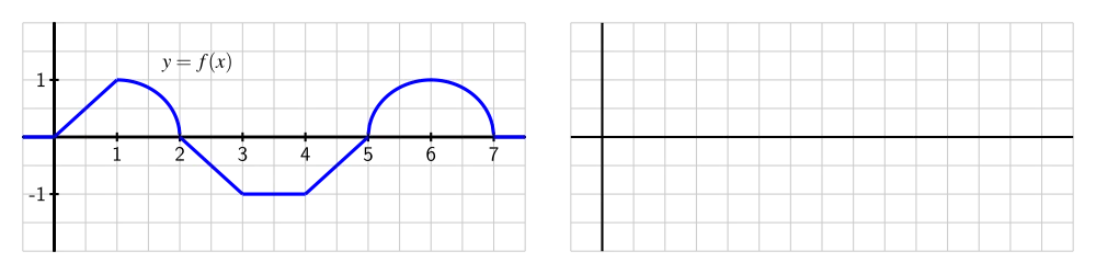
- On what interval(s) is an increasing function? On what intervals is decreasing?
- On what interval(s) is concave up? concave down? neither?
- At what point(s) does have a relative minimum? a relative maximum?
- Use the given information to determine the exact value of for In addition, what are the values of and
- Based on your responses to all of the preceding questions, sketch a complete and accurate graph of on the axes provided, being sure to indicate the behavior of for and Clearly indicate the scale on the vertical and horizontal axes of your graph.
- What happens if we change one key piece of information: in particular, say that is an antiderivative of and How (if at all) would your answers to the preceding questions change? Sketch a graph of on the same axes as the graph of you constructed in (e).
Multiple antiderivatives of a single function
In the final question of Activity , we encountered a very important idea: a function has more than one antiderivative. Each antiderivative of is determined uniquely by its value at a single point. For example, suppose that is the function given at left in Figure , and suppose further that is an antiderivative of that satisfies
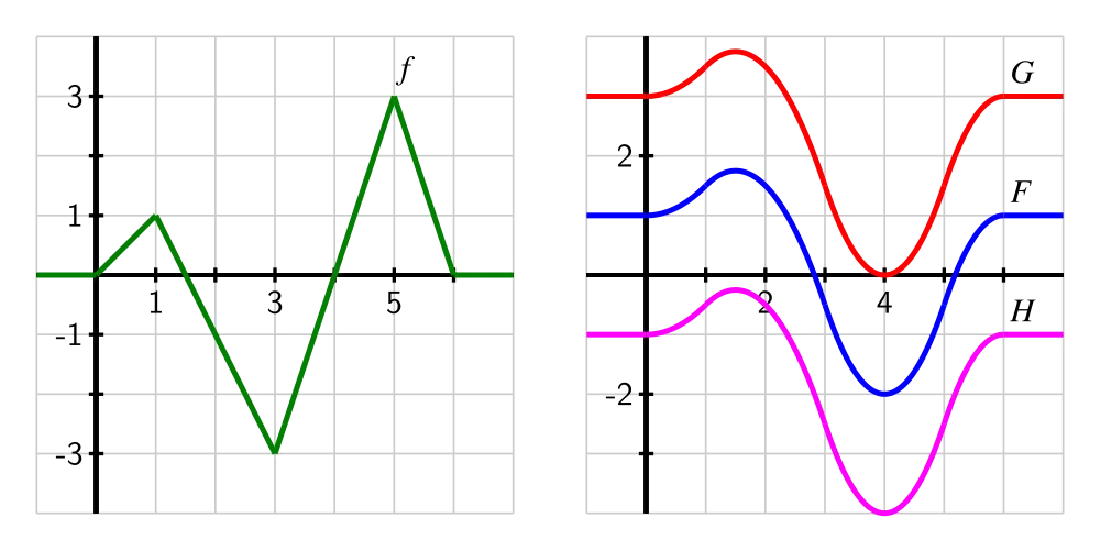
Then, using Equation (), we can compute
Similarly, and In addition, we can use the fact that to ascertain where is increasing and decreasing, concave up and concave down, and has relative extremes and inflection points. We ultimately find that the graph of is the one given in blue in Figure .
If we want an antiderivative for which then will have the exact same shape as (since both share the derivative ), but will be shifted vertically from the graph of as pictured in red in Figure . Note that just as but since whereas In the same way, if we assigned a different initial value to the antiderivative, say we would get still another antiderivative, as shown in magenta in Figure 3.
This example demonstrates an important fact that holds more generally:
Note
If and are both antiderivatives of a function then the function must be constant.
To see why this result holds, observe that if and are both antiderivatives of then and Hence,
Since the only way a function can have derivative zero is by being a constant function, it follows that the function must be constant.
We now see that if a function has at least one antiderivative, it must have infinitely many: we can add any constant of our choice to the antiderivative and get another antiderivative. For this reason, we sometimes refer to the general antiderivative of a function
To identify a particular antiderivative of we must know a single value of the antiderivative (this value is often called an initial condition). For example, if its general antiderivative is where we include the “” to indicate that includes all of the possible antiderivatives of If we know that we substitute 2 for in and find that
or Therefore, the particular antiderivative in this case is
Activity
For each of the following functions, sketch an accurate graph of the antiderivative that satisfies the given initial condition. In addition, sketch the graph of two additional antiderivatives of the given function, and state the corresponding initial conditions that each of them satisfy. If possible, find an algebraic formula for the antiderivative that satisfies the initial condition.
- original function: initial condition: interval for sketch:
- original function: initial condition: interval for sketch:
- original function: initial condition: interval for sketch:
Functions defined by integrals
Equation () allows us to compute the value of the antiderivative at a point provided that we know and can evaluate the definite integral from to of That is,
In several situations, we have used this formula to compute for several different values of and then plotted the points to help us draw an accurate graph of This suggests that we may want to think of the upper limit of integration, as a variable itself. To that end, we introduce the idea of an integral function, a function whose formula involves a definite integral.
Definition
If is a continuous function, we define the corresponding integral function according to the rule
Note that because is the independent variable in the function and determines the endpoint of the interval of integration, we need to use a different variable as the variable of integration. A standard choice is but any variable other than is acceptable.
One way to think of the function is as the “net signed area from up to ” function, where we consider the region bounded by For example, in Figure , we see a function pictured at left, and its corresponding area function (choosing ), shown at right.
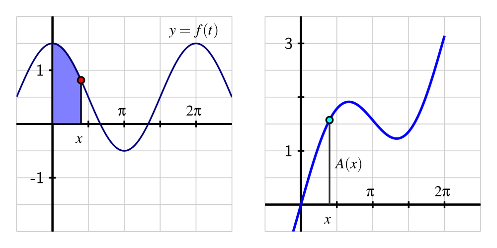
The function measures the net signed area from to bounded by the curve this value is then reported as the corresponding height on the graph of At http://gvsu.edu/s/cz, we find a java applet 1 that brings the static picture in Figure to life. There, the user can move the red point on the function and see how the corresponding height changes at the light blue point on the graph of
The choice of is somewhat arbitrary. In the activity that follows, we explore how the value of affects the graph of the integral function.
Activity
Suppose that is given by the graph at left in Figure and that is the corresponding integral function defined by
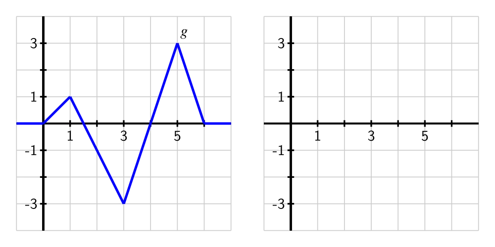
- On what interval(s) is an increasing function? On what intervals is decreasing? Why?
- On what interval(s) do you think is concave up? concave down? Why?
- At what point(s) does have a relative minimum? a relative maximum?
- Use the given information to determine the exact values of and
- Based on your responses to all of the preceding questions, sketch a complete and accurate graph of on the axes provided, being sure to indicate the behavior of for and
- How does the graph of compare to if is instead defined by
Summary
- Given the graph of a function we can construct the graph of its antiderivative provided that (a) we know a starting value of say and (b) we can evaluate the integral exactly for relevant choices of and For instance, if we wish to know we can compute When we combine this information about the function values of together with our understanding of how the behavior of affects the overall shape of we can develop a completely accurate graph of the antiderivative
- Because the derivative of a constant is zero, if is an antiderivative of it follows that will also be an antiderivative of Moreover, any two antiderivatives of a function differ precisely by a constant. Thus, any function with at least one antiderivative in fact has infinitely many, and the graphs of any two antiderivatives will differ only by a vertical translation.
- Given a function the rule defines a new function that measures the net-signed area bounded by on the interval We call the function the integral function corresponding to