Chapter 9 exercises

Exercise 9.19

Multiple regression fact checking. Determine which of the following statements are true and false. For each statement that is false, explain why it is false.

1. If predictors are collinear, then removing one variable will have no influence on the point estimate of another variable’s coefficient.

2. Suppose a numerical variable $x$ has a coefficient of $b_1 = 2.5$ in the multiple regression model. Suppose also that the first observation has $x_1 = 7.2$, the second observation has a value of $x_1 = 8.2$, and these two observations have the same values for all other predictors. Then the predicted value of the second observation will be 2.5 higher than the prediction of the first observation based on the multiple regression model.

3. If a regression model’s first variable has a coefficient of $b_1 = 5.7$, then if we are able to influence the data so that an observation will have its $x_1$ be 1 larger than it would otherwise, the value $y_1$ for this observation would increase by 5.7.

4. Suppose we fit a multiple regression model based on a data set of 472 observations. We also notice that the distribution of the residuals includes some skew but does not include any particularly extreme outliers. Because the residuals are not nearly normal, we should not use this model and require more advanced methods to model these data.

Solution in Appendix A

Exercise 9.20

Logistic regression fact checking. Determine which of the following statements are true and false. For each statement that is false, explain why it is false.

1. Suppose we consider the first two observations based on a logistic regression model, where the first variable in observation 1 takes a value of $x_1 = 6$ and observation 2 has $x_1 = 4$. Suppose we realized we made an error for these two observations, and the first observation was actually $x_1 = 7$ (instead of 6) and the second observation actually had $x_1 = 5$ (instead of 4). Then the predicted probability from the logistic regression model would increase the same amount for each observation after we correct these variables.

2. When using a logistic regression model, it is impossible for the model to predict a probability that is negative or a probability that is greater than 1.

3. Because logistic regression predicts probabilities of outcomes, observations used to build a logistic regression model need not be independent.

4. When fitting logistic regression, we typically complete model selection using adjusted $R^2$.

Exercise 9.21

Spam filtering, Part I. Spam filters are built on principles similar to those used in logistic regression. We fit a probability that each message is spam or not spam. We have several email variables for this problem: to_multiple, cc, attach, dollar, winner, inherit, password, format, re_subj, exclaim_subj, and sent_email. We won’t describe what each variable means here for the sake of brevity, but each is either a numerical or indicator variable.

1. For variable selection, we fit the full model, which includes all variables, and then we also fit each model where we’ve dropped exactly one of the variables. In each of these reduced models, the AIC value for the model is reported below. Based on these results, which variable, if any, should we drop as part of model selection? Explain.

   Variable Dropped	AIC
   None Dropped	1863.50
   to_multiple	2023.50
   cc	1863.18
   attach	1871.89
   dollar	1879.70
   winner	1885.03
   inherit	1865.55
   password	1879.31
   format	2008.85
   re_subj	1904.60
   exclaim_subj	1862.76
   sent_email	1958.18

   See the next page for part (b).

2. Consider the following model selection stage. Here again we’ve computed the AIC for each leave-one-variable-out model. Based on the results, which variable, if any, should we drop as part of model selection? Explain.

   Variable Dropped	AIC
   None Dropped	1862.41
   to_multiple	2019.55
   attach	1871.17
   dollar	1877.73
   winner	1884.95
   inherit	1864.52
   password	1878.19
   format	2007.45
   re_subj	1902.94
   sent_email	1957.56

Solution in Appendix A

Exercise 9.22

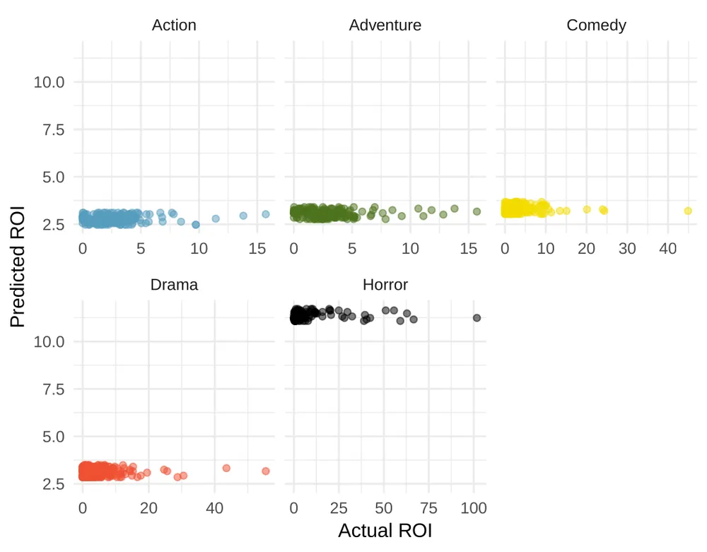
Movie returns, Part II. The student from Exercise 9.14 analyzed return-on-investment (ROI) for movies based on release year and genre of movies. The plots below show the predicted ROI vs. actual ROI for each of the genres separately. Do these figures support the comment in the FiveThirtyEight.com article that states, “The return-on-investment potential for horror movies is absurd.” Note that the x-axis range varies for each plot.

Exercise 9.23

Spam filtering, Part II. In Exercise 9.21, we encountered a data set where we applied logistic regression to aid in spam classification for individual emails. In this exercise, we’ve taken a small set of these variables and fit a formal model with the following output:

	Estimate	Std. Error	z value	Pr($>$$|$z$|$)
(Intercept)	-0.8124	0.0870	-9.34	0.0000
to_multiple	-2.6351	0.3036	-8.68	0.0000
winner	1.6272	0.3185	5.11	0.0000
format	-1.5881	0.1196	-13.28	0.0000
re_subj	-3.0467	0.3625	-8.40	0.0000

1. Write down the model using the coefficients from the model fit.

2. Suppose we have an observation where $\texttt{to\_{}multiple} = 0$, $\texttt{winner} = 1$, $\texttt{format} = 0$, and $\texttt{re\_{}subj} = 0$. What is the predicted probability that this message is spam?

3. Put yourself in the shoes of a data scientist working on a spam filter. For a given message, how high must the probability a message is spam be before you think it would be reasonable to put it in a spambox (which the user is unlikely to check)? What tradeoffs might you consider? Any ideas about how you might make your spam-filtering system even better from the perspective of someone using your email service?

Solution in Appendix A