In this section, we will introduce tables and other basic tools for categorical data that are used throughout this book. The loan50 data set represents a sample from a larger loan data set called loans. This larger data set contains information on 10,000 loans made through Lending Club. We will examine the relationship between homeownership, which for the loans data can take a value of rent, mortgage (owns but has a mortgage), or own, and app_type, which indicates whether the loan application was made with a partner or whether it was an individual application.
Contingency tables and bar plots
Figure 2.17 summarizes two variables: app_type and homeownership. A table that summarizes data for two categorical variables in this way is called a contingency table. Each value in the table represents the number of times a particular combination of variable outcomes occurred. For example, the value 3496 corresponds to the number of loans in the data set where the borrower rents their home and the application type was by an individual. Row and column totals are also included. The row totals provide the total counts across each row (e.g. ), and column totals are total counts down each column. We can also create a table that shows only the overall percentages or proportions for each combination of categories, or we can create a table for a single variable, such as the one shown in Figure 2.18 for the homeownership variable.
homeownership |
||||||
| rent | mortgage | own | Total | |||
| individual | 3496 | 3839 | 1170 | 8505 | ||
app_type |
joint | 362 | 950 | 183 | 1495 | |
| Total | 3858 | 4789 | 1353 | 10000 | ||
app_type and homeownership.homeownership |
Count |
|---|---|
| rent | 3858 |
| mortgage | 4789 |
| own | 1353 |
| Total | 10000 |
homeownership variable.A bar plot is a common way to display a single categorical variable. The left panel of Figure 2.19 shows a bar plot for the homeownership variable. In the right panel, the counts are converted into proportions, showing the proportion of observations that are in each level (e.g. for rent).
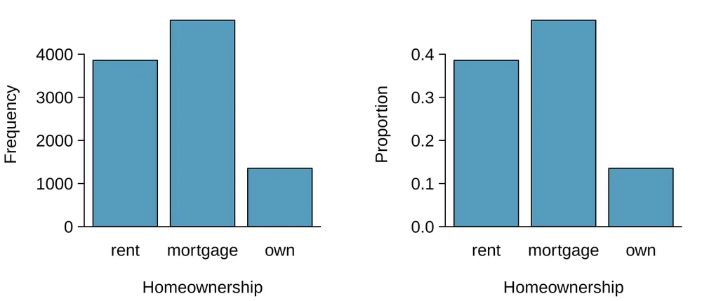
number. The left panel shows the counts, and the right panel shows the proportions in each group.Row and column proportions
Sometimes it is useful to understand the fractional breakdown of one variable in another, and we can modify our contingency table to provide such a view. Figure 2.20 shows the row proportions for Figure 2.17, which are computed as the counts divided by their row totals. The value 3496 at the intersection of individual and rent is replaced by , i.e. 3496 divided by its row total, 8505. So what does 0.411 represent? It corresponds to the proportion of individual applicants who rent.
| rent | mortgage | own | Total | |
|---|---|---|---|---|
| individual | 0.411 | 0.451 | 0.138 | 1.000 |
| joint | 0.242 | 0.635 | 0.122 | 1.000 |
| Total | 0.386 | 0.479 | 0.135 | 1.000 |
app_type and homeownership variables. The row total is off by 0.001 for the joint row due to a rounding error.A contingency table of the column proportions is computed in a similar way, where each column proportion is computed as the count divided by the corresponding column total. Figure 2.21 shows such a table, and here the value 0.906 indicates that 90.6% of renters applied as individuals for the loan. This rate is higher compared to loans from people with mortgages (80.2%) or who own their home (86.5%). Because these rates vary between the three levels of homeownership (rent, mortgage, own), this provides evidence that the app_type and homeownership variables are associated.
| rent | mortgage | own | Total | |
|---|---|---|---|---|
| individual | 0.906 | 0.802 | 0.865 | 0.851 |
| joint | 0.094 | 0.198 | 0.135 | 0.150 |
| Total | 1.000 | 1.000 | 1.000 | 1.000 |
app_type and homeownership variables. The total for the last column is off by 0.001 due to a rounding error.We could also have checked for an association between app_type and homeownership in Figure 2.20 using row proportions. When comparing these row proportions, we would look down columns to see if the fraction of loans where the borrower rents, has a mortgage, or owns varied across the individual to joint application types.
Guided Practice 2.23
(a) What does 0.451 represent in Figure 2.20?
Guided Practice 2.24
(a) What does 0.122 at the intersection of joint and own represent in Figure 2.20?
Example 2.25
Data scientists use statistics to filter spam from incoming email messages. By noting specific characteristics of an email, a data scientist may be able to classify some emails as spam or not spam with high accuracy. One such characteristic is whether the email contains no numbers, small numbers, or big numbers. Another characteristic is the email format, which indicates whether or not an email has any HTML content, such as bolded text. We’ll focus on email format and spam status using the email data set, and these variables are summarized in a contingency table in Figure 2.22. Which would be more helpful to someone hoping to classify email as spam or regular email for this table: row or column proportions?
A data scientist would be interested in how the proportion of spam changes within each email format. This corresponds to column proportions: the proportion of spam in plain text emails and the proportion of spam in HTML emails.
If we generate the column proportions, we can see that a higher fraction of plain text emails are spam () than compared to HTML emails (). This information on its own is insufficient to classify an email as spam or not spam, as over 80% of plain text emails are not spam. Yet, when we carefully combine this information with many other characteristics, we stand a reasonable chance of being able to classify some emails as spam or not spam with confidence.
| text | HTML | Total | |
|---|---|---|---|
| spam | 209 | 158 | 367 |
| not spam | 986 | 2568 | 3554 |
| Total | 1195 | 2726 | 3921 |
spam and format.Example 2.25 points out that row and column proportions are not equivalent. Before settling on one form for a table, it is important to consider each to ensure that the most useful table is constructed. However, sometimes it simply isn’t clear which, if either, is more useful.
Example 2.26
Look back to Tables 2.20 and 2.21. Are there any obvious scenarios where one might be more useful than the other?
None that we thought were obvious! What is distinct about app_type and homeownership vs the email example is that these two variables don’t have a clear explanatory-response variable relationship that we might hypothesize (see Section 1.2.4 for these terms). Usually it is most useful to “condition” on the explanatory variable. For instance, in the email example, the email format was seen as a possible explanatory variable of whether the message was spam, so we would find it more interesting to compute the relative frequencies (proportions) for each email format.
Using a bar plot with two variables
Contingency tables using row or column proportions are especially useful for examining how two categorical variables are related. Stacked bar plots provide a way to visualize the information in these tables.
A stacked bar plot
is a graphical display of contingency table information. For example, a stacked bar plot representing Figure 2.21 is shown in Figure 2.23(a), where we have first created a bar plot using the homeownership variable and then divided each group by the levels of app_type.
One related visualization to the stacked bar plot is the side-by-side bar plot, where an example is shown in Figure 2.23(b).
For the last type of bar plot we introduce, the column proportions for the app_type and homeownership contingency table have been translated into a standardized stacked bar plot in Figure 2.23(c). This type of visualization is helpful in understanding the fraction of individual or joint loan applications for borrowers in each level of homeownership. Additionally, since the proportions of joint and individual vary across the groups, we can conclude that the two variables are associated.
homeownership, where the counts have been further broken down by app_type. 2.23(b) Side-by-side bar plot for homeownership and app_type. 2.23(c) Standardized version of the stacked bar plot.Example 2.27
Examine the three bar plots in Figure 2.23(c). When is the stacked, side-by-side, or standardized stacked bar plot the most useful?
The stacked bar plot is most useful when it’s reasonable to assign one variable as the explanatory variable and the other variable as the response, since we are effectively grouping by one variable first and then breaking it down by the others.
Side-by-side bar plots are more agnostic in their display about which variable, if any, represents the explanatory and which the response variable. It is also easy to discern the number of cases in the six different group combinations. However, one downside is that it tends to require more horizontal space; the narrowness of Figure 2.23(b) makes the plot feel a bit cramped. Additionally, when two groups are of very different sizes, as we see in the own group relative to either of the other two groups, it is difficult to discern if there is an association between the variables.
The standardized stacked bar plot is helpful if the primary variable in the stacked bar plot is relatively imbalanced, e.g. the own category has only a third of the observations in the mortgage category, making the simple stacked bar plot less useful for checking for an association. The major downside of the standardized version is that we lose all sense of how many cases each of the bars represents.
Mosaic plots
A mosaic plot is a visualization technique suitable for contingency tables that resembles a standardized stacked bar plot with the benefit that we still see the relative group sizes of the primary variable as well.
To get started in creating our first mosaic plot, we’ll break a square into columns for each category of the homeownership variable, with the result shown in Figure 2.24(a). Each column represents a level of homeownership, and the column widths correspond to the proportion of loans in each of those categories. For instance, there are fewer loans where the borrower is an owner than where the borrower has a mortgage. In general, mosaic plots use box areas to represent the number of cases in each category.
homeownership. 2.24(b) Two-variable mosaic plot for both homeownership and app_type.To create a completed mosaic plot, the single-variable mosaic plot is further divided into pieces in Figure 2.24(b) using the app_type variable. Each column is split proportional to the number of loans from individual and joint borrowers. For example, the second column represents loans where the borrower has a mortgage, and it was divided into individual loans (upper) and joint loans (lower). As another example, the bottom segment of the third column represents loans where the borrower owns their home and applied jointly, while the upper segment of this column represents borrowers who are homeowners and filed individually. We can again use this plot to see that the homeownership and app_type variables are associated, since some columns are divided in different vertical locations than others, which was the same technique used for checking an association in the standardized stacked bar plot.
In Figure 2.24(b), we chose to first split by the homeowner status of the borrower. However, we could have instead first split by the application type, as in Figure 2.25. Like with the bar plots, it’s common to use the explanatory variable to represent the first split in a mosaic plot, and then for the response to break up each level of the explanatory variable, if these labels are reasonable to attach to the variables under consideration.
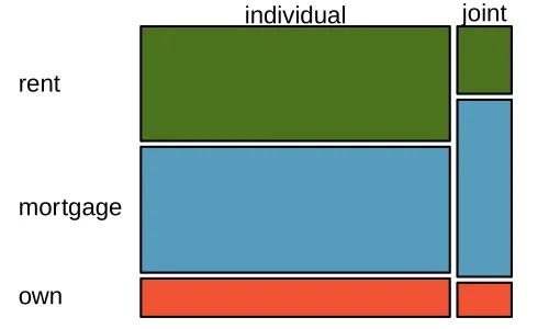
homeownership variable after they’ve been divided into the individual and joint application types.The only pie chart you will see in this book
A pie chart is shown in Figure 2.26 alongside a bar plot representing the same information. Pie charts can be useful for giving a high-level overview to show how a set of cases break down. However, it is also difficult to decipher details in a pie chart. For example, it takes a couple seconds longer to recognize that there are more loans where the borrower has a mortgage than rent when looking at the pie chart, while this detail is very obvious in the bar plot. While pie charts can be useful, we prefer bar plots for their ease in comparing groups.
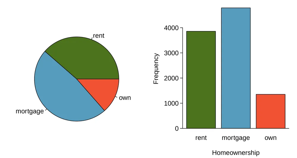
homeownership.Comparing numerical data across groups
Some of the more interesting investigations can be considered by examining numerical data across groups. The methods required here aren’t really new: all that’s required is to make a numerical plot for each group in the same graph. Here two convenient methods are introduced: side-by-side box plots and hollow histograms.
We will take a look again at the county data set and compare the median household income for counties that gained population from 2010 to 2017 versus counties that had no gain. While we might like to make a causal connection here, remember that these are observational data and so such an interpretation would be, at best, half-baked.
There were 1,454 counties where the population increased from 2010 to 2017, and there were 1,672 counties with no gain (all but one were a loss). A random sample of 100 counties from the first group and 50 from the second group are shown in Figure 2.27 to give a better sense of some of the raw median income data.
| Median Income for 150 Counties, in $1000s | |||||||||
|---|---|---|---|---|---|---|---|---|---|
| Population Gain | No Population Gain | ||||||||
| 38.2 | 43.6 | 42.2 | 61.5 | 51.1 | 45.7 | 48.3 | 60.3 | 50.7 | |
| 44.6 | 51.8 | 40.7 | 48.1 | 56.4 | 41.9 | 39.3 | 40.4 | 40.3 | |
| 40.6 | 63.3 | 52.1 | 60.3 | 49.8 | 51.7 | 57 | 47.2 | 45.9 | |
| 51.1 | 34.1 | 45.5 | 52.8 | 49.1 | 51 | 42.3 | 41.5 | 46.1 | |
| 80.8 | 46.3 | 82.2 | 43.6 | 39.7 | 49.4 | 44.9 | 51.7 | 46.4 | |
| 75.2 | 40.6 | 46.3 | 62.4 | 44.1 | 51.3 | 29.1 | 51.8 | 50.5 | |
| 51.9 | 34.7 | 54 | 42.9 | 52.2 | 45.1 | 27 | 30.9 | 34.9 | |
| 61 | 51.4 | 56.5 | 62 | 46 | 46.4 | 40.7 | 51.8 | 61.1 | |
| 53.8 | 57.6 | 69.2 | 48.4 | 40.5 | 48.6 | 43.4 | 34.7 | 45.7 | |
| 53.1 | 54.6 | 55 | 46.4 | 39.9 | 56.7 | 33.1 | 21 | 37 | |
| 63 | 49.1 | 57.2 | 44.1 | 50 | 38.9 | 52 | 31.9 | 45.7 | |
| 46.6 | 46.5 | 38.9 | 50.9 | 56 | 34.6 | 56.3 | 38.7 | 45.7 | |
| 74.2 | 63 | 49.6 | 53.7 | 77.5 | 60 | 56.2 | 43 | 21.7 | |
| 63.2 | 47.6 | 55.9 | 39.1 | 57.8 | 42.6 | 44.5 | 34.5 | 48.9 | |
| 50.4 | 49 | 45.6 | 39 | 38.8 | 37.1 | 50.9 | 42.1 | 43.2 | |
| 57.2 | 44.7 | 71.7 | 35.3 | 100.2 | 35.4 | 41.3 | 33.6 | ||
| 42.6 | 55.5 | 38.6 | 52.7 | 63 | 43.4 | 56.5 | |||
The side-by-side box plot
is a traditional tool for comparing across groups. An example is shown in the left panel of Figure 2.28, where there are two box plots, one for each group, placed into one plotting window and drawn on the same scale.
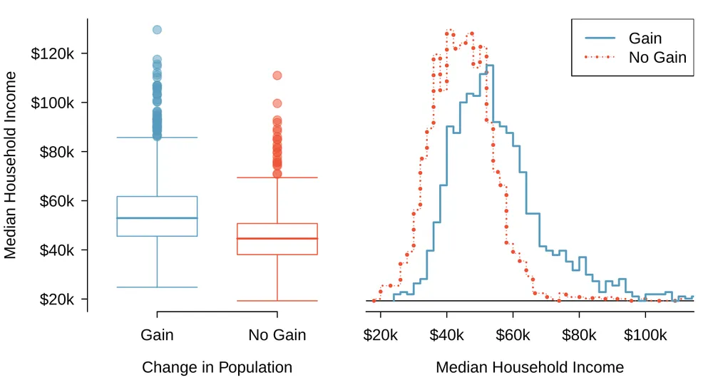
med_hh_income, where the counties are split by whether there was a population gain or there was no gain.Another useful plotting method uses hollow histograms to compare numerical data across groups. These are just the outlines of histograms of each group put on the same plot, as shown in the right panel of Figure 2.28.
Guided Practice 2.28
Use the plots in Figure 2.28 to compare the incomes for counties across the two groups. What do you notice about the approximate center of each group? What do you notice about the variability between groups? Is the shape relatively consistent between groups? How many prominent modes are there for each group?3
Exercises
Exercise 2.21
Antibiotic use in children. The bar plot and the pie chart below show the distribution of pre-existing medical conditions of children involved in a study on the optimal duration of antibiotic use in treatment of tracheitis, which is an upper respiratory infection.
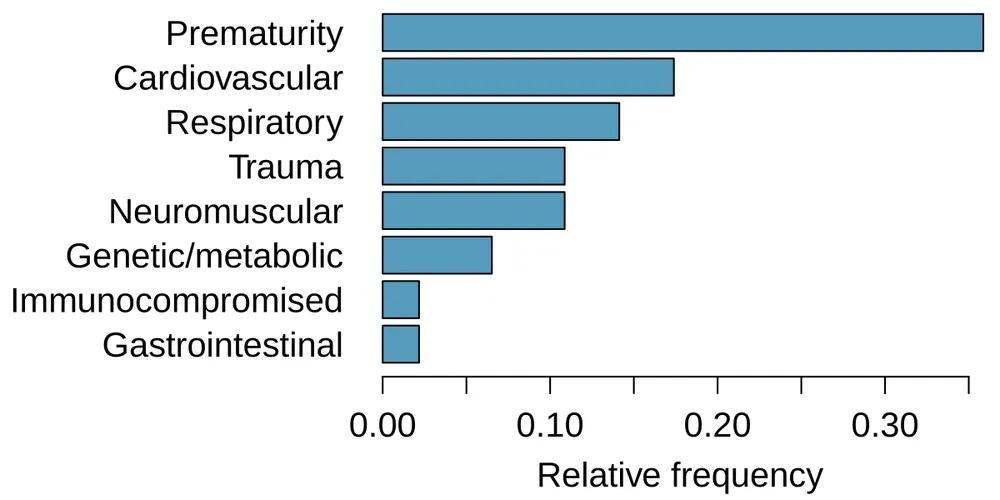
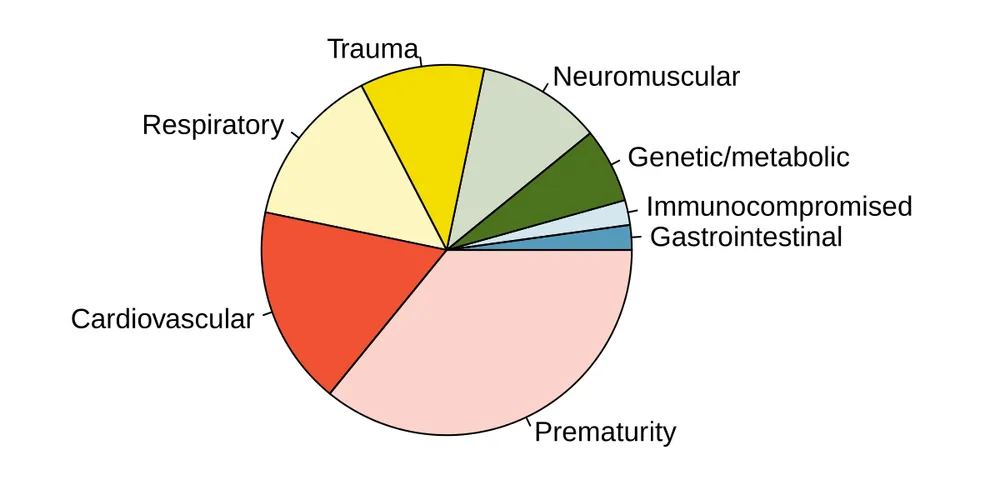
What features are apparent in the bar plot but not in the pie chart?
What features are apparent in the pie chart but not in the bar plot?
Which graph would you prefer to use for displaying these categorical data?
Exercise 2.22
Views on immigration. 910 randomly sampled registered voters from Tampa, FL were asked if they thought workers who have illegally entered the US should be (i) allowed to keep their jobs and apply for US citizenship, (ii) allowed to keep their jobs as temporary guest workers but not allowed to apply for US citizenship, or (iii) lose their jobs and have to leave the country. The results of the survey by political ideology are shown below.5
| Political ideology | |||||
| Conservative | Moderate | Liberal | Total | ||
| (i) Apply for citizenship | 57 | 120 | 101 | 278 | |
| (ii) Guest worker | 121 | 113 | 28 | 262 | |
| Response | (iii) Leave the country | 179 | 126 | 45 | 350 |
| (iv) Not sure | 15 | 4 | 1 | 20 | |
| Total | 372 | 363 | 175 | 910 | |
What percent of these Tampa, FL voters identify themselves as conservatives?
What percent of these Tampa, FL voters are in favor of the citizenship option?
What percent of these Tampa, FL voters identify themselves as conservatives and are in favor of the citizenship option?
What percent of these Tampa, FL voters who identify themselves as conservatives are also in favor of the citizenship option? What percent of moderates share this view? What percent of liberals share this view?
Do political ideology and views on immigration appear to be independent? Explain your reasoning.
Exercise 2.23
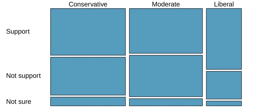
Views on the DREAM Act. A random sample of registered voters from Tampa, FL were asked if they support the DREAM Act, a proposed law which would provide a path to citizenship for people brought illegally to the US as children. The survey also collected information on the political ideology of the respondents. Based on the mosaic plot shown below, do views on the DREAM Act and political ideology appear to be independent? Explain your reasoning. 6
Exercise 2.24
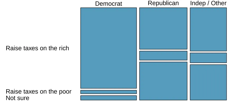
Raise taxes. A random sample of registered voters nationally were asked whether they think it’s better to raise taxes on the rich or raise taxes on the poor. The survey also collected information on the political party affiliation of the respondents. Based on the mosaic plot shown below, do views on raising taxes and political affiliation appear to be independent? Explain your reasoning. 7
Notes
(a) 0.451 represents the proportion of individual applicants who have a mortgage. (b) 0.802 represents the fraction of applicants with mortgages who applied as individuals. ↩
(a) 0.122 represents the fraction of joint borrowers who own their home. (b) 0.135 represents the home-owning borrowers who had a joint application for the loan. ↩
Answers may vary a little. The counties with population gains tend to have higher income (median of about $45,000) versus counties without a gain (median of about $40,000). The variability is also slightly larger for the population gain group. This is evident in the IQR, which is about 50% bigger in the gain group. Both distributions show slight to moderate right skew and are unimodal. The box plots indicate there are many observations far above the median in each group, though we should anticipate that many observations will fall beyond the whiskers when examining any data set that contain more than a couple hundred data points. ↩
Answers will vary. The side-by-side box plots are especially useful for comparing centers and spreads, while the hollow histograms are more useful for seeing distribution shape, skew, and potential anomalies. ↩
SurveyUSA, News Poll #18927, data collected Jan 27-29, 2012. ↩
SurveyUSA, News Poll #18927, data collected Jan 27-29, 2012. ↩
Public Policy Polling, Americans on College Degrees, Classic Literature, the Seasons, and More, data collected Feb 20-22, 2015. ↩