This chapter focuses on the mechanics and construction of summary statistics and graphs. We use statistical software for generating the summaries and graphs presented in this chapter and book. However, since this might be your first exposure to these concepts, we take our time in this chapter to detail how to create them. Mastery of the content presented in this chapter will be crucial for understanding the methods and techniques introduced in rest of the book.
In this section we will explore techniques for summarizing numerical variables. For example, consider the loan_amount variable from the loan50 data set, which represents the loan size for all 50 loans in the data set. This variable is numerical since we can sensibly discuss the numerical difference of the size of two loans. On the other hand, area codes and zip codes are not numerical, but rather they are categorical variables.
Throughout this section and the next, we will apply these methods using the loan50 and county data sets, which were introduced in Section 1.2. If you’d like to review the variables from either data set, see Figures 1.3 and 1.5.
Scatterplots for paired data
A scatterplot provides a case-by-case view of data for two numerical variables. In Figure 1.8 on Section 1.2, a scatterplot was used to examine the homeownership rate against the fraction of housing units that were part of multi-unit properties (e.g. apartments) in the county data set. Another scatterplot is shown in Figure 2.1, comparing the total income of a borrower (total_income) and the amount they borrowed (loan_amount) for the loan50 data set. In any scatterplot, each point represents a single case. Since there are 50 cases in loan50, there are 50 points in Figure 2.1.
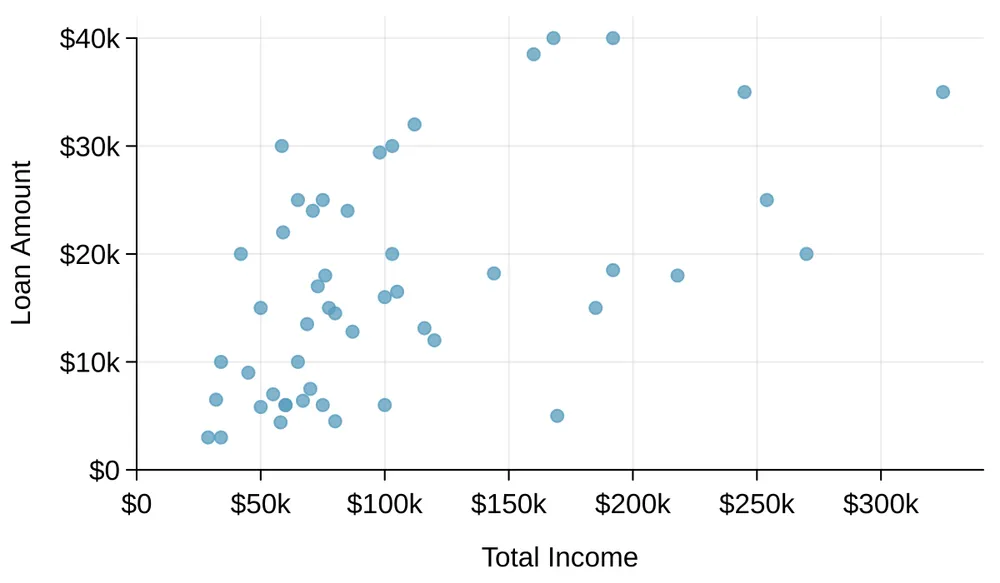
total_income versus loan_amount for the loan50 data set.Looking at Figure 2.1, we see that there are many borrowers with an income below $100,000 on the left side of the graph, while there are a handful of borrowers with income above $250,000.
Example 2.1
Figure 2.2 shows a plot of median household income against the poverty rate for 3,142 counties. What can be said about the relationship between these variables?
The relationship is evidently nonlinear, as highlighted by the dashed line. This is different from previous scatterplots we’ve seen, which show relationships that do not show much, if any, curvature in the trend.
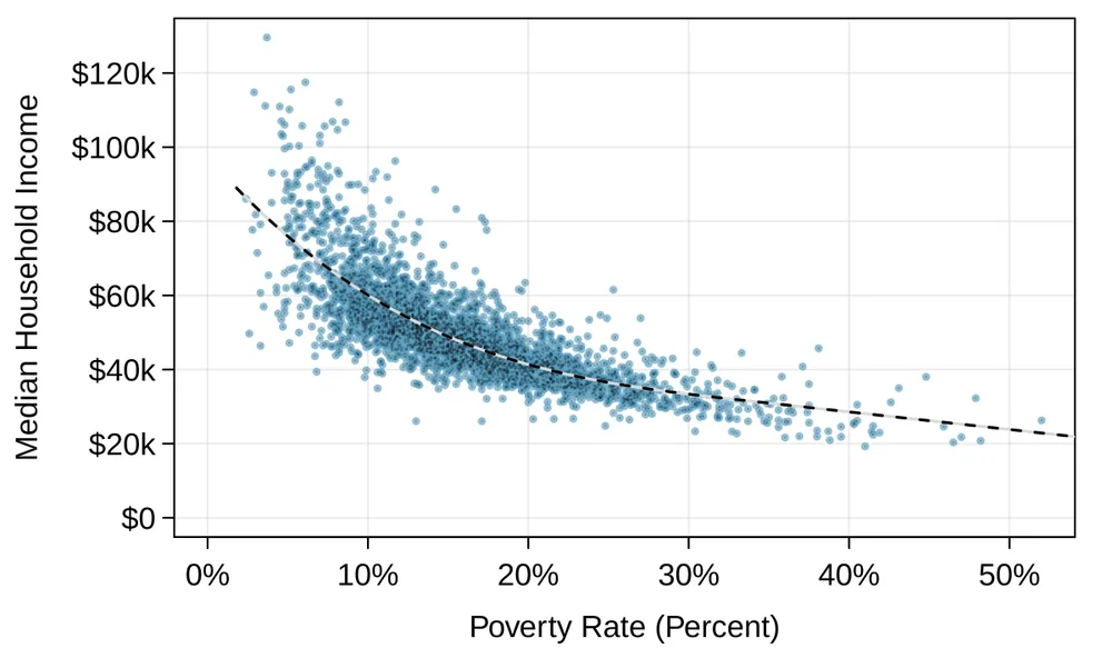
county data set. A statistical model has also been fit to the data and is shown as a dashed line.Guided Practice 2.2
What do scatterplots reveal about the data, and how are they useful?1
Guided Practice 2.3
Describe two variables that would have a horseshoe-shaped association in a scatterplot ( or ).2
Dot plots and the mean
Sometimes two variables are one too many: only one variable may be of interest. In these cases, a dot plot provides the most basic of displays. A dot plot is a one-variable scatterplot; an example using the interest rate of 50 loans is shown in Figure 2.3. A stacked version of this dot plot is shown in Figure 2.4.
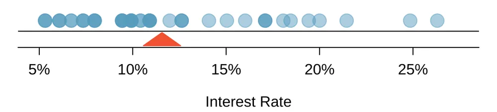
interest_rate for the loan50 data set. The distribution’s mean is shown as a red triangle.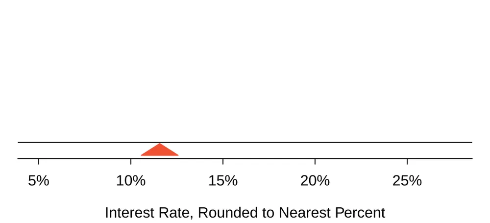
interest_rate for the loan50 data set. The rates have been rounded to the nearest percent in this plot, and the distribution’s mean is shown as a red triangle.The mean, often called the average, is a common way to measure the center of a distribution of data. To compute the mean interest rate, we add up all the interest rates and divide by the number of observations: The sample mean is often labeled . The letter is being used as a generic placeholder for the variable of interest, interest_rate, and the bar over the communicates we’re looking at the average interest rate, which for these 50 loans was 11.57%. It is useful to think of the mean as the balancing point of the distribution, and it’s shown as a triangle in Figures 2.3 and 2.4.
Mean
The sample mean can be computed as the sum of the observed values divided by the number of observations: where , , , represent the observed values.
Guided Practice 2.4
Examine the equation for the mean. What does correspond to? And ? Can you infer a general meaning to what might represent?3
Guided Practice 2.5
What was in this sample of loans?4
The loan50 data set represents a sample from a larger population of loans made through Lending Club. We could compute a mean for this population in the same way as the sample mean. However, the population mean has a special label: .
The symbol is the Greek letter mu and represents the average of all observations in the population. Sometimes a subscript, such as , is used to represent which variable the population mean refers to, e.g. . Often times it is too expensive to measure the population mean precisely, so we often estimate using the sample mean, .
Example 2.6
The average interest rate across all loans in the population can be estimated using the sample data. Based on the sample of 50 loans, what would be a reasonable estimate of , the mean interest rate for all loans in the full data set?
The sample mean, 11.57%, provides a rough estimate of . While it’s not perfect, this is our single best guess of the average interest rate of all the loans in the population under study.
In Chapter 5 and beyond, we will develop tools to characterize the accuracy of point estimates like the sample mean. As you might have guessed, point estimates based on larger samples tend to be more accurate than those based on smaller samples.
Example 2.7
The mean is useful because it allows us to rescale or standardize a metric into something more easily interpretable and comparable. Provide 2 examples where the mean is useful for making comparisons.
1. We would like to understand if a new drug is more effective at treating asthma attacks than the standard drug. A trial of 1500 adults is set up, where 500 receive the new drug, and 1000 receive a standard drug in the control group:
| New drug | Standard drug | |
|---|---|---|
| Number of patients | 500 | 1000 |
| Total asthma attacks | 200 | 300 |
Comparing the raw counts of 200 to 300 asthma attacks would make it appear that the new drug is better, but this is an artifact of the imbalanced group sizes. Instead, we should look at the average number of asthma attacks per patient in each group: The standard drug has a lower average number of asthma attacks per patient than the average in the treatment group.
2. Emilio opened a food truck last year where he sells burritos, and his business has stabilized over the last 3 months. Over that 3 month period, he has made $11,000 while working 625 hours. Emilio’s average hourly earnings provides a useful statistic for evaluating whether his venture is, at least from a financial perspective, worth it: By knowing his average hourly wage, Emilio now has put his earnings into a standard unit that is easier to compare with many other jobs that he might consider.
Example 2.8
Suppose we want to compute the average income per person in the US. To do so, we might first think to take the mean of the per capita incomes across the 3,142 counties in the county data set. What would be a better approach?
The county data set is special in that each county actually represents many individual people. If we were to simply average across the income variable, we would be treating counties with 5,000 and 5,000,000 residents equally in the calculations. Instead, we should compute the total income for each county, add up all the counties’ totals, and then divide by the number of people in all the counties. If we completed these steps with the county data, we would find that the per capita income for the US is $30,861. Had we computed the simple mean of per capita income across counties, the result would have been just $26,093!
This example used what is called a weighted mean. For more information on this topic, check out the following online supplement regarding weighted means openintro.org/d?file=stat_wtd_mean.
Histograms and shape
Dot plots show the exact value for each observation. This is useful for small data sets, but they can become hard to read with larger samples. Rather than showing the value of each observation, we prefer to think of the value as belonging to a bin. For example, in the loan50 data set, we created a table of counts for the number of loans with interest rates between 5.0% and 7.5%, then the number of loans with rates between 7.5% and 10.0%, and so on. Observations that fall on the boundary of a bin (e.g. 10.00%) are allocated to the lower bin. This tabulation is shown in Figure 2.5. These binned counts are plotted as bars in Figure 2.6 into what is called a histogram, which resembles a more heavily binned version of the stacked dot plot shown in Figure 2.4.
| Interest Rate | 5.0% - 7.5% | 7.5% - 10.0% | 10.0% - 12.5% | 12.5% - 15.0% | 25.0% - 27.5% | ||||
|---|---|---|---|---|---|---|---|---|---|
| Count | 11 | 15 | 8 | 4 | 1 |
interest_rate data.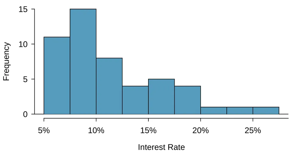
interest_rate. This distribution is strongly skewed to the right. Histograms provide a view of the data density. Higher bars represent where the data are relatively more common. For instance, there are many more loans with rates between 5% and 10% than loans with rates between 20% and 25% in the data set. The bars make it easy to see how the density of the data changes relative to the interest rate.
Histograms are especially convenient for understanding the shape of the data distribution. Figure 2.6 suggests that most loans have rates under 15%, while only a handful of loans have rates above 20%. When data trail off to the right in this way and has a longer right tail, the shape is said to be right skewed.5
Data sets with the reverse characteristic – a long, thinner tail to the left – are said to be left skewed. We also say that such a distribution has a long left tail. Data sets that show roughly equal trailing off in both directions are called symmetric.
Long tails to identify skew
When data trail off in one direction, the distribution has a long tail. If a distribution has a long left tail, it is left skewed. If a distribution has a long right tail, it is right skewed.
Guided Practice 2.9
Take a look at the dot plots in Figures 2.3 and 2.4. Can you see the skew in the data? Is it easier to see the skew in this histogram or the dot plots?6
Guided Practice 2.10
Besides the mean (since it was labeled), what can you see in the dot plots that you cannot see in the histogram?7
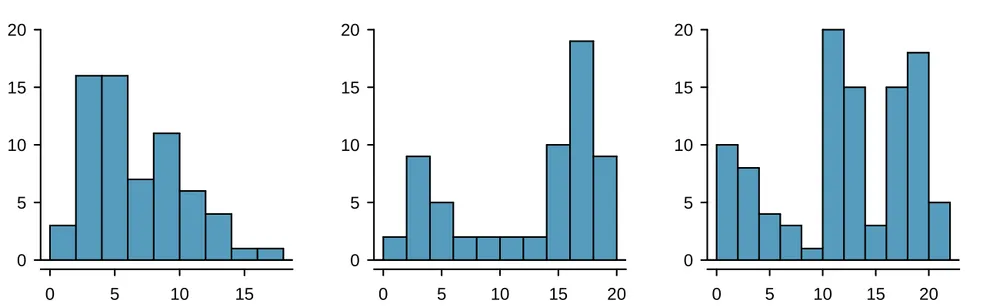
In addition to looking at whether a distribution is skewed or symmetric, histograms can be used to identify modes. A mode is represented by a prominent peak in the distribution. There is only one prominent peak in the histogram of loan_amount.
A definition of mode sometimes taught in math classes is the value with the most occurrences in the data set. However, for many real-world data sets, it is common to have no observations with the same value in a data set, making this definition impractical in data analysis.
Figure 2.7 shows histograms that have one, two, or three prominent peaks. Such distributions are called unimodal, bimodal, and multimodal, respectively. Any distribution with more than 2 prominent peaks is called multimodal. Notice that there was one prominent peak in the unimodal distribution with a second less prominent peak that was not counted since it only differs from its neighboring bins by a few observations.
Example 2.11
Figure 2.6 reveals only one prominent mode in the interest rate. Is the distribution unimodal, bimodal, or multimodal?
Unimodal. Remember that uni stands for 1 (think unicycles). Similarly, bi stands for 2 (think bicycles). We’re hoping a multicycle will be invented to complete this analogy.
Guided Practice 2.12
Height measurements of young students and adult teachers at a K-3 elementary school were taken. How many modes would you expect in this height data set?8
Looking for modes isn’t about finding a clear and correct answer about the number of modes in a distribution, which is why prominent is not rigorously defined in this book. The most important part of this examination is to better understand your data.
Variance and standard deviation
The mean was introduced as a method to describe the center of a data set, and variability in the data is also important. Here, we introduce two measures of variability: the variance and the standard deviation. Both of these are very useful in data analysis, even though their formulas are a bit tedious to calculate by hand. The standard deviation is the easier of the two to comprehend, and it roughly describes how far away the typical observation is from the mean.
We call the distance of an observation from its mean its deviation. Below are the deviations for the , , , and observations in the interest_rate variable: If we square these deviations and then take an average, the result is equal to the sample variance, denoted by : We divide by , rather than dividing by , when computing a sample’s variance; there’s some mathematical nuance here, but the end result is that doing this makes this statistic slightly more reliable and useful.
Notice that squaring the deviations does two things. First, it makes large values relatively much larger, seen by comparing , , , and . Second, it gets rid of any negative signs.
The standard deviation is defined as the square root of the variance: While often omitted, a subscript of may be added to the variance and standard deviation, i.e. and , if it is useful as a reminder that these are the variance and standard deviation of the observations represented by , , ..., .
Variance and standard deviation
The variance is the average squared distance from the mean. The standard deviation is the square root of the variance. The standard deviation is useful when considering how far the data are distributed from the mean.
The standard deviation represents the typical deviation of observations from the mean. Usually about 70% of the data will be within one standard deviation of the mean and about 95% will be within two standard deviations. However, as seen in Figures 2.8 and 2.9, these percentages are not strict rules.
Like the mean, the population values for variance and standard deviation have special symbols: for the variance and for the standard deviation. The symbol is the Greek letter sigma.
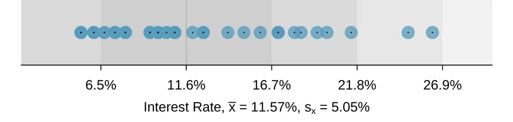
interest_rate variable, 34 of the 50 loans (68%) had interest rates within 1 standard deviation of the mean, and 48 of the 50 loans (96%) had rates within 2 standard deviations. Usually about 70% of the data are within 1 standard deviation of the mean and 95% within 2 standard deviations, though this is far from a hard rule.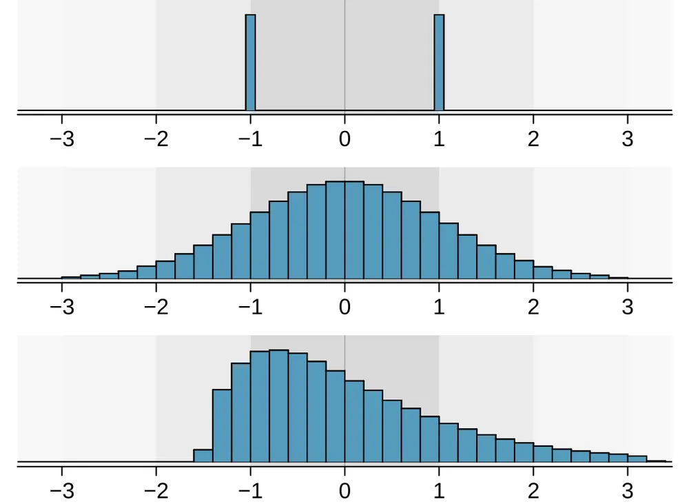
Guided Practice 2.13
In Section 2.1, the concept of shape of a distribution was introduced. A good description of the shape of a distribution should include modality and whether the distribution is symmetric or skewed to one side. Using Figure 2.9 as an example, explain why such a description is important.9
Example 2.14
Describe the distribution of the interest_rate variable using the histogram in Figure 2.6. The description should incorporate the center, variability, and shape of the distribution, and it should also be placed in context. Also note any especially unusual cases.
The distribution of interest rates is unimodal and skewed to the high end. Many of the rates fall near the mean at 11.57%, and most fall within one standard deviation (5.05%) of the mean. There are a few exceptionally large interest rates in the sample that are above 20%.
In practice, the variance and standard deviation are sometimes used as a means to an end, where the “end” is being able to accurately estimate the uncertainty associated with a sample statistic. For example, in Chapter 5 the standard deviation is used in calculations that help us understand how much a sample mean varies from one sample to the next.
Box plots, quartiles, and the median
A box plot summarizes a data set using five statistics while also plotting unusual observations. Figure 2.10 provides a vertical dot plot alongside a box plot of the interest_rate variable from the loan50 data set.
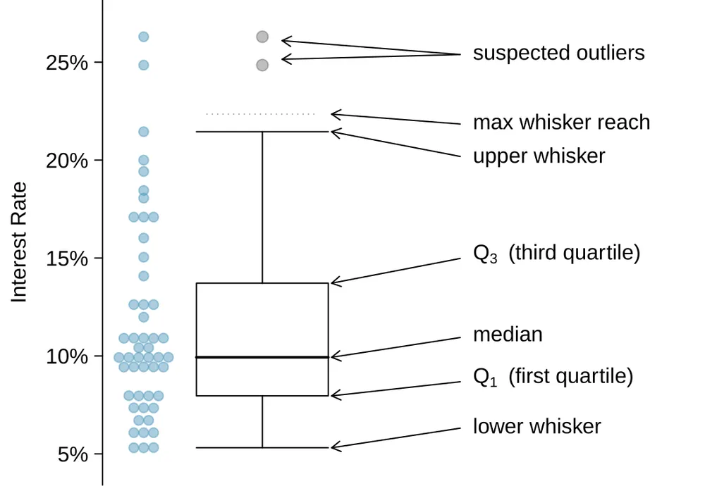
The first step in building a box plot is drawing a dark line denoting the median, which splits the data in half. Figure 2.10 shows 50% of the data falling below the median and other 50% falling above the median. There are 50 loans in the data set (an even number) so the data are perfectly split into two groups of 25. We take the median in this case to be the average of the two observations closest to the percentile, which happen to be the same value in this data set: . When there are an odd number of observations, there will be exactly one observation that splits the data into two halves, and in such a case that observation is the median (no average needed).
Median: the number in the middle
If the data are ordered from smallest to largest, the median is the observation right in the middle. If there are an even number of observations, there will be two values in the middle, and the median is taken as their average.
The second step in building a box plot is drawing a rectangle to represent the middle 50% of the data. The total length of the box, shown vertically in Figure 2.10, is called the interquartile range (IQR, for short). It, like the standard deviation, is a measure of variability in data. The more variable the data, the larger the standard deviation and IQR tend to be. The two boundaries of the box are called the first quartile (the percentile, i.e. 25% of the data fall below this value) and the third quartile (the percentile), and these are often labeled and , respectively.
Interquartile range (IQR)
The IQR is the length of the box in a box plot. It is computed as where and are the and percentiles.
Guided Practice 2.15
What percent of the data fall between and the median? What percent is between the median and ?10
Extending out from the box, the whiskers attempt to capture the data outside of the box. However, their reach is never allowed to be more than . They capture everything within this reach. In Figure 2.10, the upper whisker does not extend to the last two points, which is beyond , and so it extends only to the last point below this limit. The lower whisker stops at the lowest value, 5.31%, since there is no additional data to reach; the lower whisker’s limit is not shown in the figure because the plot does not extend down to . In a sense, the box is like the body of the box plot and the whiskers are like its arms trying to reach the rest of the data.
Any observation lying beyond the whiskers is labeled with a dot. The purpose of labeling these points – instead of extending the whiskers to the minimum and maximum observed values – is to help identify any observations that appear to be unusually distant from the rest of the data. Unusually distant observations are called outliers. In this case, it would be reasonable to classify the interest rates of 24.85% and 26.30% as outliers since they are numerically distant from most of the data.
Outliers are extreme
An outlier is an observation that appears extreme relative to the rest of the data.
Examining data for outliers serves many useful purposes, including
Identifying strong skew in the distribution.
Identifying possible data collection or data entry errors.
Providing insight into interesting properties of the data.
Guided Practice 2.16
Using Figure 2.10, estimate the following values for interest_rate in the loan50 data set:
(a) , (b) , and (c) IQR.11
Robust statistics
How are the sample statistics of the interest_rate data set affected by the observation, 26.3%? What would have happened if this loan had instead been only 15%? What would happen to these summary statistics if the observation at 26.3% had been even larger, say 35%? These scenarios are plotted alongside the original data in Figure 2.11, and sample statistics are computed under each scenario in Figure 2.12.
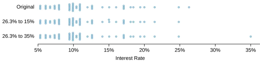
| robust | not robust | |||||
|---|---|---|---|---|---|---|
| scenario | median | IQR | ||||
original interest_rate data |
9.93% | 5.76% | 11.57% | 5.05% | ||
| move 26.3% 15% | 9.93% | 5.76% | 11.34% | 4.61% | ||
| move 26.3% 35% | 9.93% | 5.76% | 11.74% | 5.68% | ||
interest_rate variable been different.Guided Practice 2.17
(a) Which is more affected by extreme observations, the mean or median? Figure 2.12 may be helpful. (b) Is the standard deviation or IQR more affected by extreme observations?12
The median and IQR are called robust statistics because extreme observations have little effect on their values: moving the most extreme value generally has little influence on these statistics. On the other hand, the mean and standard deviation are more heavily influenced by changes in extreme observations, which can be important in some situations.
Example 2.18
The median and IQR did not change under the three scenarios in Figure 2.12. Why might this be the case?
The median and IQR are only sensitive to numbers near , the median, and . Since values in these regions are stable in the three data sets, the median and IQR estimates are also stable.
Guided Practice 2.19
The distribution of loan amounts in the loan50 data set is right skewed, with a few large loans lingering out into the right tail. If you were wanting to understand the typical loan size, should you be more interested in the mean or median?13
Transforming data (special topic)
data are very strongly skewed, we sometimes transform them so they are easier to model.
Example 2.20
Consider the histogram of county populations shown in Figure 2.13(a), which shows extreme skew. What isn’t useful about this plot?
Nearly all of the data fall into the left-most bin, and the extreme skew obscures many of the potentially interesting details in the data.
There are some standard transformations that may be useful for strongly right skewed data where much of the data is positive but clustered near zero. A transformation is a rescaling of the data using a function. For instance, a plot of the logarithm (base 10) of county populations results in the new histogram in Figure 2.13(b). This data is symmetric, and any potential outliers appear much less extreme than in the original data set. By reigning in the outliers and extreme skew, transformations like this often make it easier to build statistical models against the data.
Transformations can also be applied to one or both variables in a scatterplot. A scatterplot of the population change from 2010 to 2017 against the population in 2010 is shown in Figure 2.14(a). In this first scatterplot, it’s hard to decipher any interesting patterns because the population variable is so strongly skewed. However, if we apply a log transformation to the population variable, as shown in Figure 2.14(b), a positive association between the variables is revealed. In fact, we may be interested in fitting a trend line to the data when we explore methods around fitting regression lines in Chapter 8.
Transformations other than the logarithm can be useful, too. For instance, the square root () and inverse () are commonly used by data scientists. Common goals in transforming data are to see the data structure differently, reduce skew, assist in modeling, or straighten a nonlinear relationship in a scatterplot.
Mapping data (special topic)
The county data set offers many numerical variables that we could plot using dot plots, scatterplots, or box plots, but these miss the true nature of the data. Rather, when we encounter geographic data, we should create an intensity map, where colors are used to show higher and lower values of a variable. Figures 2.15(b) and 2.16(b) shows intensity maps for poverty rate in percent (poverty), unemployment rate (unemployment_rate), homeownership rate in percent (homeownership), and median household income (median_hh_income). The color key indicates which colors correspond to which values. The intensity maps are not generally very helpful for getting precise values in any given county, but they are very helpful for seeing geographic trends and generating interesting research questions or hypotheses.
Example 2.21
What interesting features are evident in the poverty and unemployment_rate intensity maps?
Poverty rates are evidently higher in a few locations. Notably, the deep south shows higher poverty rates, as does much of Arizona and New Mexico. High poverty rates are evident in the Mississippi flood plains a little north of New Orleans and also in a large section of Kentucky.
The unemployment rate follows similar trends, and we can see correspondence between the two variables. In fact, it makes sense for higher rates of unemployment to be closely related to poverty rates. One observation that stand out when comparing the two maps: the poverty rate is much higher than the unemployment rate, meaning while many people may be working, they are not making enough to break out of poverty.
Guided Practice 2.22
What interesting features are evident in the median_hh_income intensity map in Figure 2.16(b)?14
Exercises
Exercise 2.1
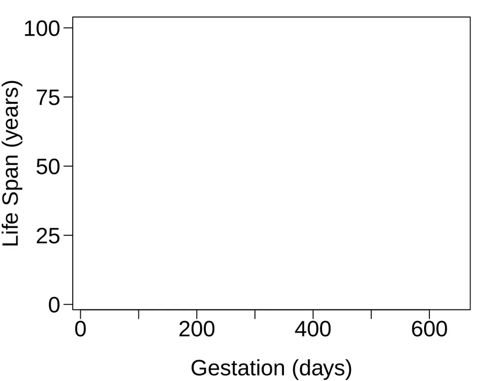
Mammal life spans. Data were collected on life spans (in years) and gestation lengths (in days) for 62 mammals. A scatterplot of life span versus length of gestation is shown below. 15
What type of an association is apparent between life span and length of gestation?
What type of an association would you expect to see if the axes of the plot were reversed, i.e. if we plotted length of gestation versus life span?
Are life span and length of gestation independent? Explain your reasoning.
Exercise 2.2
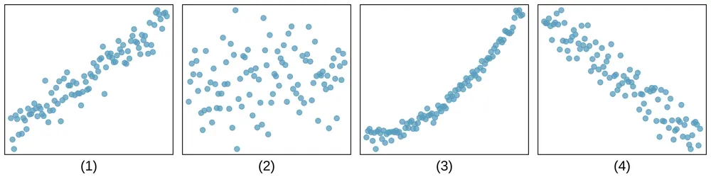
Associations. Indicate which of the plots show (a) a positive association, (b) a negative association, or (c) no association. Also determine if the positive and negative associations are linear or nonlinear. Each part may refer to more than one plot.
Exercise 2.3
Reproducing bacteria. Suppose that there is only sufficient space and nutrients to support one million bacterial cells in a petri dish. You place a few bacterial cells in this petri dish, allow them to reproduce freely, and record the number of bacterial cells in the dish over time. Sketch a plot representing the relationship between number of bacterial cells and time.
Exercise 2.4
Office productivity. Office productivity is relatively low when the employees feel no stress about their work or job security. However, high levels of stress can also lead to reduced employee productivity. Sketch a plot to represent the relationship between stress and productivity.
Exercise 2.5
Parameters and statistics. Identify which value represents the sample mean and which value represents the claimed population mean.
American households spent an average of about $52 in 2007 on Halloween merchandise such as costumes, decorations and candy. To see if this number had changed, researchers conducted a new survey in 2008 before industry numbers were reported. The survey included 1,500 households and found that average Halloween spending was $58 per household.
The average GPA of students in 2001 at a private university was 3.37. A survey on a sample of 203 students from this university yielded an average GPA of 3.59 a decade later.
Exercise 2.6
Sleeping in college. A recent article in a college newspaper stated that college students get an average of 5.5 hrs of sleep each night. A student who was skeptical about this value decided to conduct a survey by randomly sampling 25 students. On average, the sampled students slept 6.25 hours per night. Identify which value represents the sample mean and which value represents the claimed population mean.
Exercise 2.7
Days off at a mining plant. Workers at a particular mining site receive an average of 35 days paid vacation, which is lower than the national average. The manager of this plant is under pressure from a local union to increase the amount of paid time off. However, he does not want to give more days off to the workers because that would be costly. Instead he decides he should fire 10 employees in such a way as to raise the average number of days off that are reported by his employees. In order to achieve this goal, should he fire employees who have the most number of days off, least number of days off, or those who have about the average number of days off?
Exercise 2.8
Medians and IQRs. For each part, compare distributions (1) and (2) based on their medians and IQRs. You do not need to calculate these statistics; simply state how the medians and IQRs compare. Make sure to explain your reasoning.
(1) 3, 5, 6, 7, 9
(2) 3, 5, 6, 7, 20(1) 3, 5, 6, 7, 9
(2) 3, 5, 7, 8, 9(1) 1, 2, 3, 4, 5
(2) 6, 7, 8, 9, 10(1) 0, 10, 50, 60, 100
(2) 0, 100, 500, 600, 1000
Exercise 2.9
Means and SDs. For each part, compare distributions (1) and (2) based on their means and standard deviations. You do not need to calculate these statistics; simply state how the means and the standard deviations compare. Make sure to explain your reasoning. Hint: It may be useful to sketch dot plots of the distributions.
(1) 3, 5, 5, 5, 8, 11, 11, 11, 13
(2) 3, 5, 5, 5, 8, 11, 11, 11, 20
(1) -20, 0, 0, 0, 15, 25, 30, 30
(2) -40, 0, 0, 0, 15, 25, 30, 30(1) 0, 2, 4, 6, 8, 10
(2) 20, 22, 24, 26, 28, 30(1) 100, 200, 300, 400, 500
(2) 0, 50, 300, 550, 600
Exercise 2.10
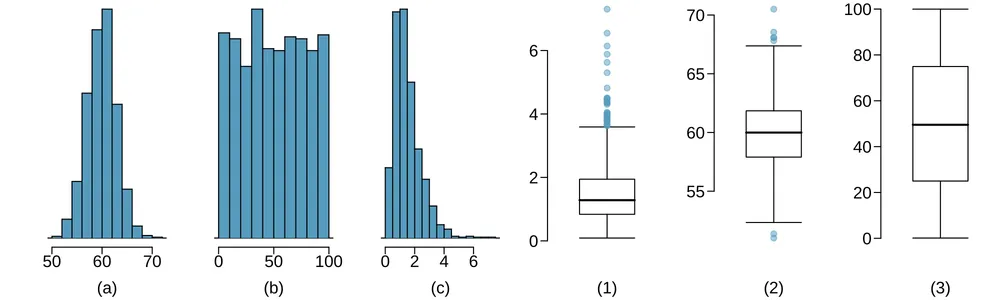
Mix-and-match. Describe the distribution in the histograms below and match them to the box plots.
Exercise 2.11
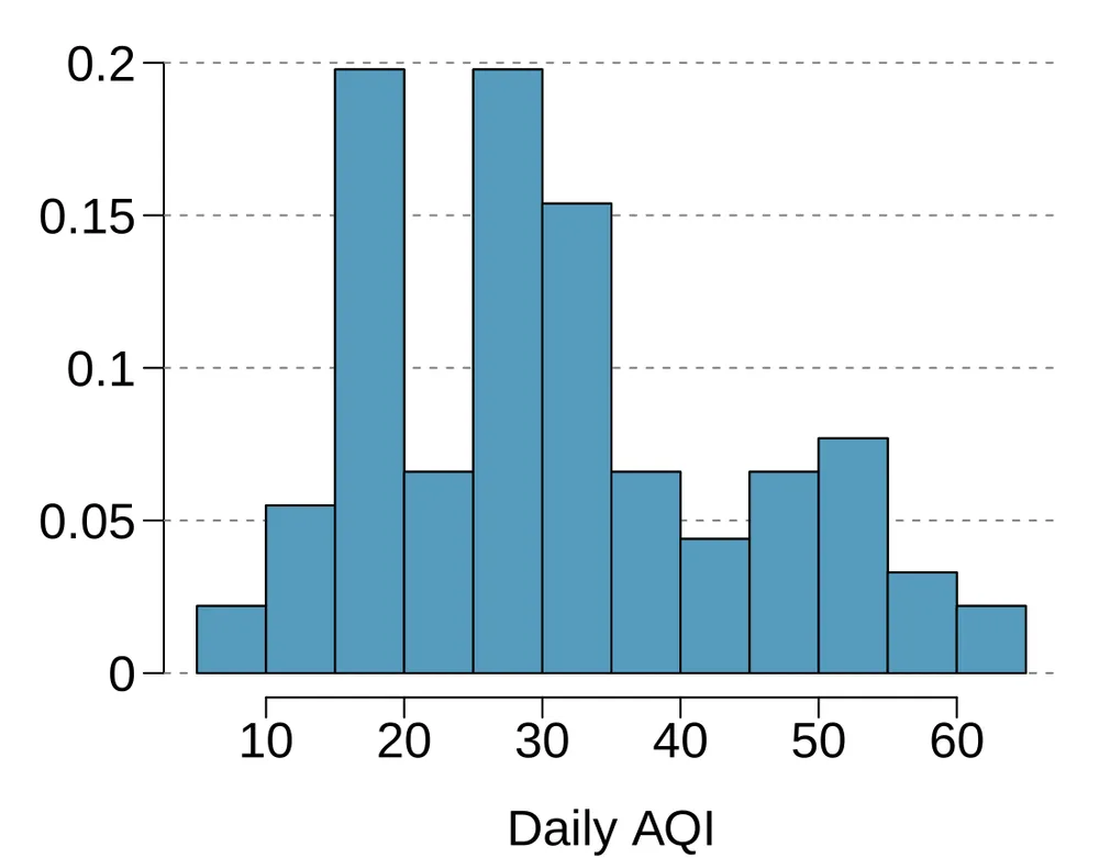
Air quality. Daily air quality is measured by the air quality index (AQI) reported by the Environmental Protection Agency. This index reports the pollution level and what associated health effects might be a concern. The index is calculated for five major air pollutants regulated by the Clean Air Act and takes values from 0 to 300, where a higher value indicates lower air quality. AQI was reported for a sample of 91 days in 2011 in Durham, NC. The relative frequency histogram below shows the distribution of the AQI values on these days. 16
Estimate the median AQI value of this sample.
Would you expect the mean AQI value of this sample to be higher or lower than the median? Explain your reasoning.
Estimate Q1, Q3, and IQR for the distribution.
Would any of the days in this sample be considered to have an unusually low or high AQI? Explain your reasoning.
Exercise 2.12
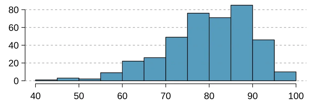
Median vs. mean. Estimate the median for the 400 observations shown in the histogram, and note whether you expect the mean to be higher or lower than the median.
Exercise 2.13
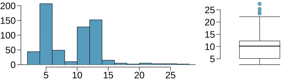
Histograms vs. box plots. Compare the two plots below. What characteristics of the distribution are apparent in the histogram and not in the box plot? What characteristics are apparent in the box plot but not in the histogram?
Exercise 2.14
Facebook friends. Facebook data indicate that 50% of Facebook users have 100 or more friends, and that the average friend count of users is 190. What do these findings suggest about the shape of the distribution of number of friends of Facebook users? 17
Exercise 2.15
Distributions and appropriate statistics, Part I. For each of the following, state whether you expect the distribution to be symmetric, right skewed, or left skewed. Also specify whether the mean or median would best represent a typical observation in the data, and whether the variability of observations would be best represented using the standard deviation or IQR. Explain your reasoning.
Number of pets per household.
Distance to work, i.e. number of miles between work and home.
Heights of adult males.
Exercise 2.16
Distributions and appropriate statistics, Part II. For each of the following, state whether you expect the distribution to be symmetric, right skewed, or left skewed. Also specify whether the mean or median would best represent a typical observation in the data, and whether the variability of observations would be best represented using the standard deviation or IQR. Explain your reasoning.
Housing prices in a country where 25% of the houses cost below $350,000, 50% of the houses cost below $450,000, 75% of the houses cost below $1,000,000 and there are a meaningful number of houses that cost more than $6,000,000.
Housing prices in a country where 25% of the houses cost below $300,000, 50% of the houses cost below $600,000, 75% of the houses cost below $900,000 and very few houses that cost more than $1,200,000.
Number of alcoholic drinks consumed by college students in a given week. Assume that most of these students don’t drink since they are under 21 years old, and only a few drink excessively.
Annual salaries of the employees at a Fortune 500 company where only a few high level executives earn much higher salaries than all the other employees.
Exercise 2.17
Income at the coffee shop. The first histogram below shows the distribution of the yearly incomes of 40 patrons at a college coffee shop. Suppose two new people walk into the coffee shop: one making $225,000 and the other $250,000. The second histogram shows the new income distribution. Summary statistics are also provided.
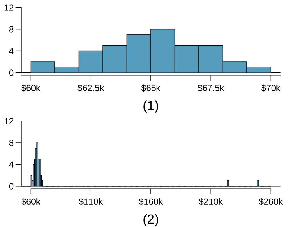
| (1) | (2) | |
|---|---|---|
| n | 40 | 42 |
| Min. | 60,680 | 60,680 |
| 1st Qu. | 63,620 | 63,710 |
| Median | 65,240 | 65,350 |
| Mean | 65,090 | 73,300 |
| 3rd Qu. | 66,160 | 66,540 |
| Max. | 69,890 | 250,000 |
| SD | 2,122 | 37,321 |
Would the mean or the median best represent what we might think of as a typical income for the 42 patrons at this coffee shop? What does this say about the robustness of the two measures?
Would the standard deviation or the IQR best represent the amount of variability in the incomes of the 42 patrons at this coffee shop? What does this say about the robustness of the two measures?
Exercise 2.18
Midrange. The midrange of a distribution is defined as the average of the maximum and the minimum of that distribution. Is this statistic robust to outliers and extreme skew? Explain your reasoning
Exercise 2.19
Commute times. The US census collects data on time it takes Americans to commute to work, among many other variables. The histogram below shows the distribution of average commute times in 3,142 US counties in 2010. Also shown below is a spatial intensity map of the same data.
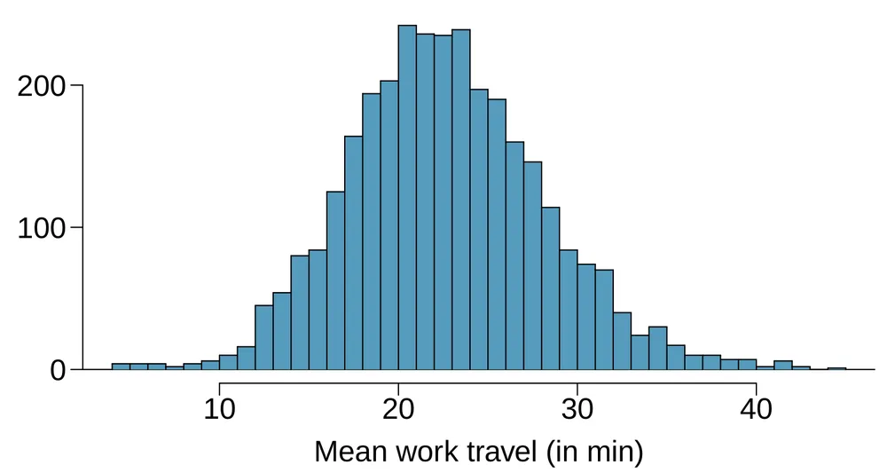
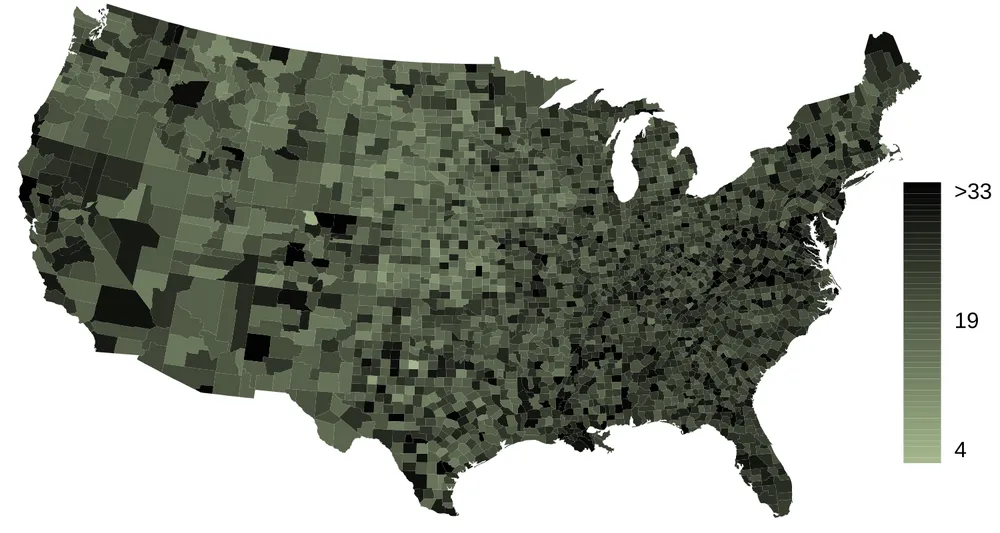
Describe the numerical distribution and comment on whether or not a log transformation may be advisable for these data.
Describe the spatial distribution of commuting times using the map above.
Exercise 2.20
Hispanic population. The US census collects data on race and ethnicity of Americans, among many other variables. The histogram below shows the distribution of the percentage of the population that is Hispanic in 3,142 counties in the US in 2010. Also shown is a histogram of logs of these values.
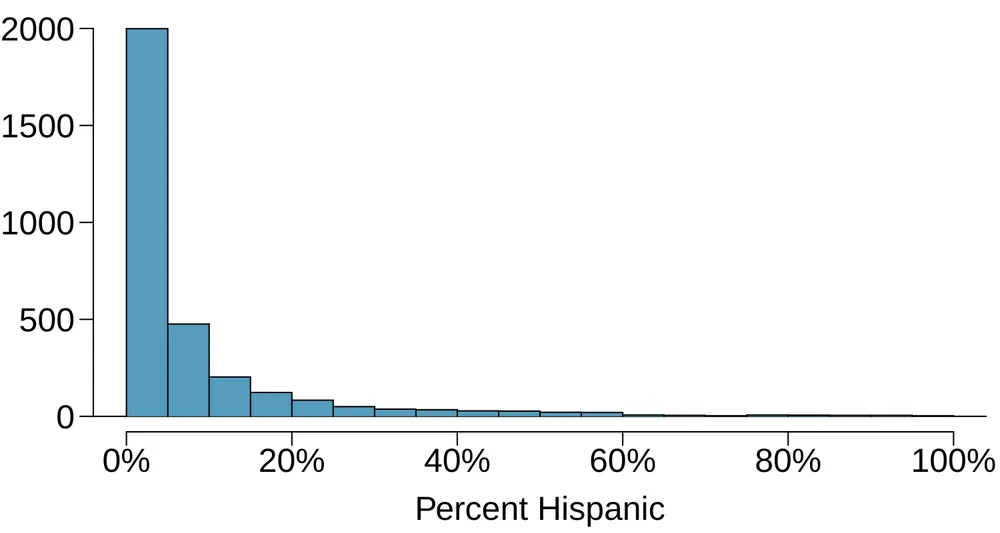
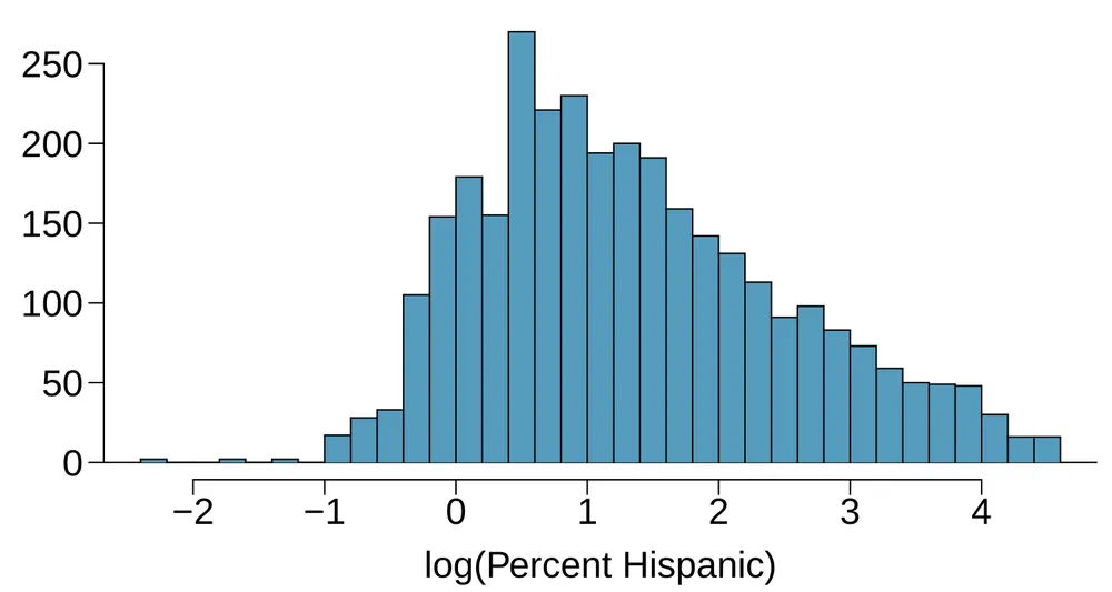
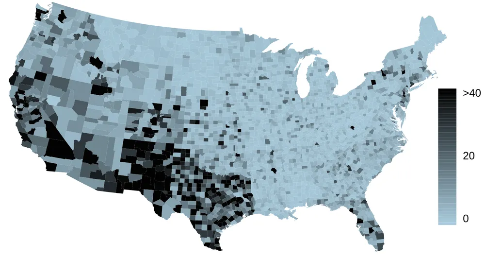
Describe the numerical distribution and comment on why we might want to use log-transformed values in analyzing or modeling these data.
What features of the distribution of the Hispanic population in US counties are apparent in the map but not in the histogram? What features are apparent in the histogram but not the map?
Is one visualization more appropriate or helpful than the other? Explain your reasoning.
Notes
Answers may vary. Scatterplots are helpful in quickly spotting associations relating variables, whether those associations come in the form of simple trends or whether those relationships are more complex. ↩
Consider the case where your vertical axis represents something “good” and your horizontal axis represents something that is only good in moderation. Health and water consumption fit this description: we require some water to survive, but consume too much and it becomes toxic and can kill a person. ↩
corresponds to the interest rate for the first loan in the sample (10.90%), to the second loan’s interest rate (9.92%), and corresponds to the interest rate for the loan in the data set. For example, if , then we’re examining , which refers to the fourth observation in the data set. ↩
The sample size was . ↩
Other ways to describe data that are right skewed: skewed to the right, skewed to the high end, or skewed to the positive end. ↩
The skew is visible in all three plots, though the flat dot plot is the least useful. The stacked dot plot and histogram are helpful visualizations for identifying skew. ↩
The interest rates for individual loans. ↩
There might be two height groups visible in the data set: one of the students and one of the adults. That is, the data are probably bimodal. ↩
Figure 2.9 shows three distributions that look quite different, but all have the same mean, variance, and standard deviation. Using modality, we can distinguish between the first plot (bimodal) and the last two (unimodal). Using skewness, we can distinguish between the last plot (right skewed) and the first two. While a picture, like a histogram, tells a more complete story, we can use modality and shape (symmetry/skew) to characterize basic information about a distribution. ↩
Since and capture the middle 50% of the data and the median splits the data in the middle, 25% of the data fall between and the median, and another 25% falls between the median and . ↩
These visual estimates will vary a little from one person to the next: 8%, 14%, . (The true values: , , .) ↩
(a) Mean is affected more. (b) Standard deviation is affected more. Complete explanations are provided in the material following Guided Practice 2.17. ↩
Answers will vary! If we’re looking to simply understand what a typical individual loan looks like, the median is probably more useful. However, if the goal is to understand something that scales well, such as the total amount of money we might need to have on hand if we were to offer 1,000 loans, then the mean would be more useful. ↩
Note: answers will vary. There is some correspondence between high earning and metropolitan areas, where we can see darker spots (higher median household income), though there are several exceptions. You might look for large cities you are familiar with and try to spot them on the map as dark spots. ↩
Allison, T. and Cicchetti, D.V. Sleep in mammals: ecological and constitutional correlates. Arch. Hydrobiol. 1975. ↩
US Environmental Protection Agency, AirData, 2011.. ↩
Backstrom, Lars. Anatomy of Facebook. Facebook Data Team’s Notes. 2011. ↩